In a fast-flux service network, the hosts associated with a domain name are constantly ... scams or malicious web content that attempts to infect the end user.
MISHIMA: Multilateration of Internet hosts hidden using malicious fast-flux agents (Short Paper) Greg Banks, Aristide Fattori, Richard Kemmerer, Christopher Kruegel, and Giovanni Vigna University of California, Santa Barbara {nomed,joystick,kemm,chris,vigna}@cs.ucsb.edu Abstract. Fast-flux botnets are a growing security concern on the Internet. At their core, these botnets are a large collection of geographicallydispersed, compromised machines that act as proxies to hide the location of the host, commonly referred to as the “mothership,” to/from which they are proxying traffic. Fast-flux botnets pose a serious problem to botnet take-down efforts. The reason is that, while it is typically easy to identify and consequently shut down single bots, locating the mothership behind a cloud of dynamically changing proxies is a difficult task. This paper presents techniques that utilize characteristics inherent in fast-flux service networks to thwart the very purpose for which they are used. Namely, we leverage the geographically-dispersed set of proxy hosts to locate (multilaterate) the position of the mothership in an abstract ndimensional space. In this space, the distance between a pair of network coordinates is the round-trip time between the hosts they represent in the network. To map network coordinates to actual IP addresses, we built an IP graph that models the Internet. In this IP graph, nodes are Class C subnets and edges are routes between these subnets. By combining information obtained by calculating network coordinates and the IP graph, we are able to establish a group of subnets to which a mothership likely belongs.
1
Introduction
In recent years, there has been a dramatic change in the goals and modes of operation of malicious hackers. As hackers have realized the potential monetary gains associated with Internet fraud, there has been a shift from “hacking for fun” [1] to “hacking for profit” [2]. As part of this shift, cybercriminals realized that it was necessary to create large-scale infrastructures to provide services (e.g., spam delivery) and protect important parts of their operations from identification and countermeasures. To this end, botnets and fast-flux networks were introduced. Botnets are sets of compromised hosts (usually thousands) that are under the control of an attacker, who can then use them to provide services and perform distributed attacks. Hosts in a botnet can also be used as reverse web proxies to serve the content of malicious web sites. In this case, the proxying bots are usually organized as a fast-flux service network [3].
In a fast-flux service network, the hosts associated with a domain name are constantly changed to make it harder to block the delivery of the malicious web pages and effectively hide the address of the actual web server, often referred to as the “mothership.” A number of countermeasures against botnets have been proposed, but none of these is able to address the problem of identifying the location of mothership hosts with good approximation. In this paper, we present a novel approach that utilizes characteristics inherent in fast-flux service networks to thwart the very purpose for which they are used. Namely, we leverage the geographically-dispersed set of proxy hosts in order to multilaterate (more commonly, and mistakenly, referred to as “triangulate”) the position of the mothership host in an abstract n-dimensional space. In this space, the distance between a pair of coordinates is the round-trip time between the hosts they represent in the network. Unfortunately, calculating the network coordinates of a host does not give any information about its IP address. To overcome this limitation, we built an IP graph that models the Internet. In this graph, nodes represent Class C subnets and edges represent routes between these subnets. This IP graph is then used to map network coordinates to a set of likely IP addresses. This leads to a significant reduction of the effort needed to shutdown a fast-flux botnet’s mothership. This paper makes the following two main contributions: (i) we introduce a novel approach to compute the location of a mothership host that is hidden behind a fast-flux service network; (ii) we create an IP graph representing a model of the Internet topology, which allows us to map network coordinates to actual Class C subnets.
2
Background and Related Work
Given the continuous rise in malicious botnet activity, there has been a significant amount of recent work both in botnet analysis and botnet mitigation. Analysis efforts [2, 4, 5] have attempted to quantify the number and sizes of botnets. As for mitigation, researchers examined the life cycle of bots [6] and, in particular, the command and control (C&C) channels that are used to exchange information between a botmaster and the infected machines. 2.1
Fast-Flux Service Networks
A particularly troubling development related to botnets is the advent of fast-flux service networks. In a nutshell, fast-flux service networks utilize existing botnets to hide a particular resource or server. This server is generally a host to phishing scams or malicious web content that attempts to infect the end user. Two types of fast-flux networks have been observed in the wild: single-flux and double-flux. In single-flux networks, the DNS A records for a domain are constantly updated with the addresses of bots that act as reverse proxies for the content associated with the domain. Double-flux networks add a second layer of redirection to this scheme. In these networks, the NS records associated with the authoritative name servers for a malicious domain are also short-lived and rotated.
Much of the work involving fast-flux networks has been related to detection and understanding. Holz et al. identify the issue and suggest metrics for detection [7]. The authors characterize fast-flux service networks and introduce a function to calculate the “flux-score” for a domain. Similarly, Passerini et al. developed a tool, called FluXOR, to detect and monitor fast-flux service networks [8]. Nazario et al. use a globally distributed set of honeypots to collect suspect domains, which are then analyzed according to a set of heuristics and identified as being hosted by a fast-flux service network or not [9]. Even though the approaches mentioned above represent a fundamental step toward understanding and detecting fast-flux networks, none of them is able to determine or characterize the location of a mothership. Thus, they assume that the fast-flux service network provides an impenetrable cloaking mechanism to the mothership host. 2.2
Network Coordinates
While fast-flux networks are able to hide much about the mothership, they still expose round-trip times and provide a large number of beacons (e.g., bots acting as reverse proxies) through which to communicate. Similar prerequisites (i.e., beacons and a distance metric) are necessary for systems dealing with location estimation, such as GPS, triangulation, and multilateration, all of which have an Internet counterpart: network coordinate systems. Techniques dealing with network coordinate systems were first developed to predict Internet latencies. One of the early approaches to predict latency between hosts was a service called IDMaps [10]. The problem with this method is that it requires an additional underlying infrastructure for which the end user is just a client. Ng and Zhang proposed a different method, called global network positioning (GNP), by which Internet hosts interested in latency prediction would interactively participate to create a model of the network as a 3-dimensional Euclidean space [11]. Given this model, each host in the network is assigned a set of coordinates. Latency estimation then becomes a simple calculation of Euclidean distance given the coordinates of two hosts. In 2004, Dabek et al. developed a network coordinate system called Vivaldi, which is based on GNP [12]. Vivaldi describes the network as a series of nodes connected by springs and tries to minimize the energy in this network. In this way, each node in the network has a push or pull effect on neighboring nodes and the system settles or converges on a set of coordinates that accurately predicts latencies. Costa et al. developed the PIC algorithm around the same time as Vivaldi [13]. PIC also builds on GNP using the same idea of a multi-dimensional space to model network latencies. A concurrent work by Castelluccia et al. was developed simultaneously to MISHIMA [14]. The technique presented in this work aims at geolocalizing proxied services, with a particular focus on fast-flux hidden servers. Their approach is somewhat similar to ours, as they also use multilateration of Internet hosts, but we believe their technique to be both less precise and less complete. The reason is that they can only give an idea of the geographical location of a fastflux server with an approximation of 100 km2 or more. This makes it difficult to actually identify the network location (IP address) of a host and the network carrier responsible for take-down.
3
Approach
We developed a system, called MISHIMA (Multilateration of Internet hostS Hidden usIng Malicious fast-flux Agents), to actively calculate the coordinates of motherships associated with various domains that have been identified as being hosted by fast-flux service networks. Our main goal in doing this is to determine the location of a mothership, where by “location,” we mean a Class C subnet (or a set of them) to which the mothership likely belongs. Our approach to fast-flux mothership multilateration works in three steps: In the first step, we make use of existing network coordinate calculation techniques to determine the coordinates of the various proxies, or bots, that are part of a proxy network for a particular fast-flux domain. The coordinates of a proxy (or, in general, any host) represent a point in an n-dimensional Euclidean space where the measure of distance between hosts is their round-trip time (RTT). In the second step, we utilize three characteristics of fast-flux service networks in order to multilaterate the position of the mothership that is used to host the actual content for a domain. In the third step, we use network coordinates and attempt to map them to IP addresses, using a network model of the Internet. 3.1
Calculation of Proxy Network Coordinates
We calculate the network coordinates for the proxies of a fast-flux service network using the algorithm by Costa et al. [13], while incorporating ideas by Gummadi et al. [15] and Ledlie et al. [16]. Costa et al. provide a general algorithm to calculate the network coordinates for hosts in an n-dimensional space given the measurement of actual round-trip times between hosts. The goal of the coordinate system is to be able to estimate the latency between two hosts whose coordinates are known, by calculating the Euclidean distance between the coordinates. This means that two nodes who lie close to each other in the coordinate space are likely in the same network, while those that lie far away from each other are likely in different networks. Network coordinate systems require a large number of geographically-dispersed beacons to perform well [11]. A legitimate resource available to the research community that fits these characteristics is PlanetLab. Therefore, we make use of approximately 150-200 PlanetLab nodes distributed throughout North America, Europe, and Asia at any given time. For our system, we need to know the coordinates of these beacons as well as their distance from a target (which we get using various probing techniques). We have created a centralized database containing a large number of coordinates. This allows us to do a simple linear scan over the appropriate nodes to find the closest ones. In the case that we have no coordinates for a particular target, we have to estimate them before we can actually find their closest nodes. To this end, we first use random nodes (beacons) to estimate the coordinates of the target, and then scan the database of known coordinates to find beacons that are close to it. In addition to having a large number of geographically-dispersed beacons, we also need a supply of malicious domains to work with. To this end, we utilize
two sources: the Arbor Networks Atlas repository [17] and a locally-collected repository of domains harvested from the .COM zone file. The DNS resource records for each domain are checked against a simple set of heuristics throughout the process to determine whether they are still hosted by fast-flux networks. The heuristics used are as follows: – – – –
There must be at least nine distinct A records associated with the domain. The TTL associated with each record must be less than 1,000 seconds. The percentage of A records from the same /16 must be less than 70. The NS records for a query must not belong to a small blacklist of those used to “park” domains.
Unlike most network coordinates studies, we have very specific constraints on our ability to probe the machines whose coordinates we want to calculate. Traditionally, latency measurements are performed using ICMP echo probes or some application-level probe (usually UDP-based), in the case that ICMP probes are filtered. For our purposes, we use directed TCP-based application-level probes in the case of both fast-flux agents and mothership network coordinate calculations, and ICMP-based echo probes for our PlanetLab (beacon) nodes. In fact, we have to use TCP-based probes in the case of the proxy agents for two reasons: first, since most of the fast-flux agents reside in residential and DHCP assigned networks, ICMP ping probes are filtered; second, we need a way to measure the round-trip-time from the proxy node to the mothership. To calculate the RTT to the mothership, we measure the RTT to the proxy as the time difference from the outgoing TCP packet containing the GET request to its respective ACK. The RTT from the proxy to the mothership is the time difference between the outgoing GET request and the incoming HTTP response minus the RTT to the proxy node. To calculate the network coordinates for a target given the RTTs extracted from our probes, we use the Nelder-Mead simplex method using the sum of the squared relative errors between the actual distance and the predicted distance as the objective function to be minimized. 3.2
Mothership Network Coordinate Calculation
We calculate the network coordinates for a mothership by leveraging a sideeffect of the first step. More precisely, in calculating the network coordinates for a fast-flux proxy node we are also able to estimate the RTT to the mothership from the proxy. Since we can estimate the RTT from a proxy to the mothership and we are able to calculate the coordinates of hundreds, or even thousands, of proxies associated with a particular mothership, we satisfy the two prerequisites for multilateration: (1) a significant number of geographically-dispersed beacon nodes, and (2) distance measurements from those beacons to the node whose coordinates are unknown. By doing this, we can use the algorithm by Costa et al. [13] using these proxies and their RTTs as input. We need to calculate the coordinates for at least sixteen proxies before we attempt to calculate the coordinates of a mothership. In our implementation, we
consider a domain ready for mothership multilateration when we have calculated the coordinates for at least 100 proxies. This gives us enough beacons to calculate at least eight coordinates for the mothership using the hybrid approach in [13], the flexibility to choose a varied set of beacons, and the opportunity to discard outliers. 3.3
IP Graph
Even if it is possible to determine the network coordinates of a mothership, this information does not allow one to directly determine the corresponding IP address. Therefore, we need a way to map the network coordinates of a host to its IP address (or a set of likely IP addresses). To do this, we first build an IP graph. In this graph, nodes are Class C subnets and edges represent routes between these subnets. To build the IP graph, we made use of the CAIDA topology datasets [18]. This data is generated through the use of geographically-distributed machines that continuously calculate routes toward a large set of hosts, and it is made available daily, thus granting very up-to-date data. To create our graph, we parse all CAIDA data but we take into consideration only Class C subnets, as routing information within the same subnet is too fine-grained for our purposes. Once the IP graph has been built, we pre-compute the network coordinates for a large number of IP addresses on the Internet. Then, given the network coordinates of a particular machine of interest, we can find all nodes in the IP graph that have close (pre-computed) network coordinates. After that, we use the IP graph (and its edges) to look for other nodes that are close. These nodes represent likely Class C networks where the machine of interest is located. More precisely, the algorithm works as follows: We first calculate the set K of the n nearest networks to the target t, of which we only know the network coordinates NC. To determine which networks are in this set, we calculate the Euclidean distance between every node in the IP graph G and NC, and we pick the n closest nodes. Then, for each k ∈ K, we compute the set of nodes that are reachable from k via a maximum number d of hops in G, and we call these sets of close nodes candidate sets Ck . Finally, we create the set K ′ that contains only the nodes that appear in a certain percentage p of the candidate sets Ck generated during the previous step. Of course, K ′ will contain some nodes that are far away from t. We prune these nodes by eliminating all nodes that are farther away from t than a given threshold. In Figure 1, we show a simple example of this technique applied to a small partition of the graph. Assume t is our target, d = 2, p = 1 (100%), and the set of closest nodes, based only on the Euclidean distance computed from network coordinates, is K := {a, b, c}. As we explained before, we take every element of K, and, for each element, we find all the nodes in G that are a maximum number of hops d away. This results in the new sets Ca , Cb , and Cc , marked in the example with a dotted, a full, and a dashed line, respectively. We then compute the intersection of these three sets. In these example, the result is the set K ′ := {a, t}. In real-world cases, the sets Ck can become quite large. For this reason, as we will show in Section 4, a choice of p < 1 leads to better results.
Cb b
t a
c
Ca
Cc Fig. 1. From Network Coordinates to Subnet(s)
4
Experimental Results
In a first test, we picked a set of known hosts (targets). We then computed their network coordinates and evaluated the effectiveness of our approach to map these network coordinates back to IP addresses. More precisely, we applied our technique to eight distinct hosts, using different settings for p (the fraction of candidate sets in which a Class C network must appear before it is reported in the results). A larger value of p results in fewer networks that are reported (that is, the result set is tighter). On the other hand, it is also more likely that the true location of a host is missed. All experiments have been performed with n = 10, d = 2, and threshold = 10.
Target
128.111.4.0 128.111.4.0 128.111.4.0 128.111.4.0 114.108.44.0 114.108.44.0 114.108.44.0 114.108.44.0 85.17.143.0 85.17.143.0 85.17.143.0 85.17.143.0 59.136.176.0 59.136.176.0 59.136.176.0 59.136.176.0
p
100% 50% 30% 10% 100% 50% 30% 10% 100% 50% 30% 10% 100% 50% 30% 10%
Intersection Found Target
p
2 X 159.149.153.0 100% 75 X 159.149.153.0 50% 75 X 159.149.153.0 30% 75 X 159.149.153.0 10% 0 99.54.140.0 100% 6 99.54.140.0 50% 54 X 99.54.140.0 30% 77 X 99.54.140.0 10% 1 114.108.82.0 100% 48 X 114.108.82.0 50% 48 X 114.108.82.0 30% 82 X 114.108.82.0 10% 0 93.160.107.1 100% 149 X 93.160.107.1 50% 196 X 93.160.107.1 30% 222 X 93.160.107.1 10% Table 1. Real-World Experiments
Intersection Found
0 2 31 31 0 0 0 1 0 6 71 71 0 2 10 115
X X
X X
X
In Table 1, we report the results of our experiments. For each target host, we show the percentage of candidate sets to which a node (network) must belong to be reported in the detection results (column p) as well as the number of Class C networks that appear in the result set (column intersection). We also report whether the true target was part of the result set. From Table 1, we can see that a value of p = 30 seems to offer a good tradeoff between detection and precision. That is, in 6 out of 8 cases, the true location of the network was detected, and the number of potential Class C networks is typically less than a hundred. It is interesting to note that we are not able to find any non-empty intersection (except for p = 10%) when looking for the target subnet 99.54.140.0/24. We investigated the reason for this, and we discovered that we have very little knowledge of the network coordinates of nodes close to this subnet. Because of this, the elements belonging to the set of closest nodes are at a medium distance of 30 from the target, while in the other successful cases we have a medium distance between 0.5 and 8. Therefore, knowing the network coordinates of hosts in the neighborhood of the target is a prerequisite to be able to determine a set of nodes to which the target likely belongs. We also performed our tests with different parameter settings for the number of initial nodes n, the distance d, and the threshold t. For space reasons, we can discuss these results only briefly. When using d = 3 instead of d = 2, the results remain similar, but the precision starts to decrease and the result sets grow. Also, changing the initial number of near nodes n does not improve the results significantly. The most interesting parameter was the threshold value. Indeed, by using a threshold smaller than 10, we can reduce the size of the intersection considerably. For example, with a threshold = 2, we can prune the intersection to two nodes, or even to one, and still find our target. However, we decided to use a more conservative approach (threshold = 10) since, in the case of real-world motherships, we have to take into account noise. We also investigated how many different Autonomous Systems (AS) cover the subnets in the resulting intersection. Our findings are encouraging. In fact, in most of our experiments, all of the subnets contained in the intersection belong to the same AS. This can help in obtaining a more precise identification of the mothership, as, once we discover the AS to which the mothership belongs, it could be possible to start a collaboration with the corresponding ISP or institution to analyze network traffic or to perform scanning in the AS network in order to detect the mothership with greater precision. To demonstrate the effectiveness of our approach on a real-world botnet, we decided to analyze the then-active Waledac botnet. To do this, we fed four fastflux domains associated with this botnet to MISHIMA and we identified 335 hosts that are acting as proxies for its mothership. Next, we calculated their network coordinates and ran the IP detection algorithm. This yielded 48 Class C subnets where the mothership was likely located. To confirm our result, we set up a honeypot Windows XP machine and infected it with the latest sample of the malware associated with Waledac. To get the most up to date sample, we retrieved it directly from botnet hosts that are serving it. By doing this, we were able to infiltrate the botnet and discover the mothership IP address. We were able to successfully confirm that the actual mothership was in one of the
48 networks that we found. We want to point out that the knowledge of the IP address of the mothership has been used only to validate our results and not, in any way, to determine the set where the mothership might have been located.
5
Attacks & Shortcomings
There are several ways in which a knowledgeable attacker might try to prevent the correct identification of the mothership’s location. First, fast-flux proxies could artificially delay the HTTP responses that we require for our probes, thus invalidating our coordinate calculations. If this delay were a static value, our coordinates would simply represent a point far away in the coordinate space from the actual coordinates. If the delay was random, we would only be able to calculate the general area where the mothership would likely lie. Over the course of our measurements, we did not see anything that indicated this behavior was taking place. Second, since we are heavily reliant on a relatively large number of probes to each beacon, we cannot deal with proxies that recognize this behavior and cease to proxy connections. We saw this behavior with some domains (e.g., a request to a domain from the same IP address within a few-minutes period would only return the malicious web page for the first several requests). The most likely method to mitigate this attack would be to throttle our probes to an appropriate speed. Third, there are several network topologies that would confuse our measurements and invalidate the coordinates we calculate. If the proxies are set up to load-balance requests among a number of motherships, we will most likely calculate incorrect, or at least inconsistent, coordinates. Currently, we assume that there is exactly one mothership. If this is not the case, the RTTs associated with our probes will conflict, and our results will likely resemble those in the case of random artificial delay being inserted into our probes. Even though it may be possible to identify and cluster RTTs in an effort to identify those that were destined for a different mothership, we did not see results that indicated that load-balancing was being performed.
6
Conclusions
We have presented MISHIMA, a system that helps to automatically identify and cluster fast-flux hosted domains by their respective motherships. By integrating our knowledge of network coordinates and of the Internet topology, we are able to determine a set of subnets to which the mothership likely belongs. Last but not least, MISHIMA goes beyond previous heuristic-based approaches to mothership clustering and makes use of more robust characteristics at the network and application level, allowing it to identify motherships in spite of the presence of different fast-flux service networks and disparate web content. In conclusion, we believe that MISHIMA will constitute a useful contribution to the efforts undertaken to counteract the threat of fast-flux botnets.
References 1. Bailey, M., Cooke, E., Jahanian, F., Watson, D., Nazario, J.: The Blaster Worm: Then and Now. IEEE Security & Privace (2005) 26–31 2. Cooke, E., Jahanian, F., McPherson, D.: The Zombie Roundup: Understanding, Detecting, and Disrupting Botnets. In: Proceedings of the USENIX SRUTI Workshop. (2005) 39–44 3. The Honeynet Project: Know Your Enemy: Fast-Flux Service Networks. www. honeynet.org/book/export/html/130 (2007) 4. Freiling, F., Holz, T., Wicherski, G.: Botnet Tracking: Exploring a Root-Cause Methodology to Prevent Distributed Denial-of-Service Attacks. In: 10th European Symposium On Research In Computer Security. (2005) 5. Rajab, M.A., Zarfoss, J., Monrose, F., Terzis, A.: A Multifaceted Approach to Understanding the Botnet Phenomenon. In: 6th ACM SIGCOMM Internet Measurement Conference (IMC). (2006) 6. Gu, G., Porras, P., Yegneswaran, V., Fong, M., Lee, W.: BotHunter: Detecting Malware Infection Through IDS-Driven Dialog Correlation. In: Proceedings of the 16th USENIX Security Symposium. (2007) 7. Holz, T., Gorecki, C., Rieck, K., Freiling, F.C.: Measuring and detecting fast-flux service networks. In: Network & Distributed System Security Symposium. (2008) 8. Passerini, E., Paleari, R., Martignoni, L., Bruschi, D.: FluXOR: Detecting and Monitoring Fast-Flux Service Networks. Lecture Notes in Computer Science (2008) 9. Nazario, J., Holz, T.: As the Net Churns: Fast-Flux Botnet Observations. In: Conference on Malicious and Unwanted Software (Malware’08). (2008) 10. Francis, P., Jamin, S., Jin, C., Jin, Y., Raz, D., Shavitt, Y., Zhang, L.: IDMaps: A Global Internet Host Distance Estimation Service. IEEE/ACM TRANSACTIONS ON NETWORKING 9(5) (2001) 525 11. Ng, T., Zhang, H.: Towards global network positioning. In: Proceedings of the 1st ACM SIGCOMM Workshop on Internet Measurement, ACM New York, NY, USA (2001) 25–29 12. Dabek, F., Cox, R., Kaashoek, F., Morris, R.: Vivaldi: a decentralized network coordinate system. ACM SIGCOMM Computer Communication Review 34(4) (2004) 15–26 13. Costa M. and Castro M. and Rowstron R. and Key P.: PIC: Practical Internet Coordinates for Distance Estimation. In: Proceedings of the International Conference on Distributed Computing Systems. (2004) 178–187 14. C. Castelluccia, D. Kaafar, P., Perito, D.: Geolocalization of Proxied Services and its Application to Fast-Flux Hidden Servers. In: 9th ACM SIGCOMM Internet Measurement Conference (IMC). (2009) 15. Gummadi, K., Saroiu, S., Gfibble, S.: King: Estimating Latency between Arbitrary Internet End Hosts. In: Proceedings of SIGCOMM Workshop on Internet Measurment. (2002) 5–18 16. Ledlie, J., Gardner, P., Seltzer, M.: Network Coordinates in the Wild. In: Proceedings of USENIX NSDI. (April 2007) 17. Arbor Networks: Arbor Atlas http://atlas.arbor.net. 18. Y. Hyun, B. Huffaker, D. Andersen, E. Aben, C. Shannon, M. Luckie, and kc claffy: The CAIDA IPv4 Routed /24 Topology Dataset. http://www.caida.org/data/ active/ipv4 routed 24 topology dataset.xml (07/2009-09/2009)