Sep 2, 2011 - proaches to improve fidelity of Global Positioning System ..... FAA/Ohio University LAAS Program Review, Power Point Presentation.
19th European Signal Processing Conference (EUSIPCO 2011)
Barcelona, Spain, August 29 - September 2, 2011
MITIGATION OF GPS PERIODIC MULTIPATH USING NONLINEAR REGRESSION Quoc-Huy Phan, Su-Lim Tan School of Computer Engineering, Nanyang Technological University 50 Nanyang Ave, Singapore 639798 email: {phan0035, assltan}@ntu.edu.sg
ABSTRACT Motivated by the idea of imposing machine learning approaches to improve fidelity of Global Positioning System (GPS) measurements, this work proposes a nonlinear regression method to tackle multipath mitigation problem for GPS fixed ground stations. Posing multipath error corresponding to each visible satellite as a function of the satellite’s repeatable geometry with respect to a fixed receiver on sidereal daily basis, the multipath estimator is trained using historical data of a few reference days and is then used to correct multipath-corrupted measurements on the successive days. The well-known Support Vector Regression (SVR) is employed to train the estimator of multipath of each satellite. With error analysis on real recorded data, we show that our proposed method achieve state-of-the-art performance in code multipath mitigation with 79% reduction on average in terms of standard deviation of multipath error. The improvement on precision of positioning solution of multipathcorrected data is of 25-35%. 1. INTRODUCTION GPS multipath is defined as one or more indirect replicas of line-of-sight signals received by the antenna from reflected objects in its surroundings. Among variety of error sources contaminating receivers’ measurements, multipath disturbance remains a major error impairing accuracy and precision of GPS positioning. Firstly, multipath error typically causes range error up to 15 meters for code measurements [2] and a few centimeters for carrier-phase measurements [3]. These range errors are intolerated for high-precision applications. Secondly, multipath noise is environment-dependent; implying no correlation between multipath occurring at an end of GPS baseline and that one at the other end. Thus, the differential GPS which is employed to minimize the spatially correlated error like tropospheric delay, ionospheric delay, etc., does not work on multipath. Therefore, reduction of multipath becomes essential for high-precision GPS applications. Many approaches have been previously developed for multipath mitigation. They can be classified into 3 categories: radio frequency (RF), receiver-based and postreception data processing approaches. RF approaches involve multipath-rejecting antenna design techniques to attenuate the undesired multipath signals before they enter receivers [5], site selection to avoid obstacles [6] or using electromagnetic fences [7] to minimize multipath signals. Receiver-based approaches employ advanced correlator design techniques in receiver tracking loops to minimize multipath for code measurements [8] and carrier phase measurements [9]. Despite the techniques of two foregoing categories are applied; in practice, the range error induced by remaining multipath is still large at observable level [2, 3]
© EURASIP, 2011 - ISSN 2076-1465
as previously mentioned. Hence, various post-reception data processing techniques have been proposed for supplementarily reduction of remaining multipath. These approaches can be further classified as frequency-domain and time-domain processing. As the former is concerned, based on spectrum analysis of code-minus-carrier (CmC) sequence, multipath errors can be minimized by nulling out the spectrum in its bounded frequency region [10]. Multipath signature can also be extracted with wavelet decomposition, which then can be directly applied to remove multipath errors from subsequent measurements [11, 12]. However, correcting multipath noise on frequency domain may affect other secondary signals that are derived to study other phenomena like earthquake, etc. as their spectrum may overlap with the spectrum of multipath. An approach adopting signal-to-noise measurement as a measure of precision of carrier-phase measurements to weight each receiver-satellite pair [13, 14]; unfortunately, they are not always available in RINEX observation file which makes it inapplicable in many situations. Regarding to time domain processing methods, the typical technique is carrier smoothing filter (CSF) [1] to average out noisy code measurements with precise but ambiguous carrier phase measurements. Still, CSF is effective to reduce receiver noise and very high-frequency multipath error for a given smoothing window width but less operative for lower frequency multipath error [10]. A major trend in timedomain processing is the modeling approach which takes advantage of repeatability of multipath sequences on daily basis of a fixed station to stack multiple multipath sequences of consecutive days [4, 15, 16]. The stacked multipath sequences are then time-shifted with repeatable period to calibrate multipath error for subsequent measurements. However, it is not obvious which time shift to use since different satellites are visible at different times of the day and they orbit the earth with slightly different periods. Following this trend, this work suggests a novel non-parametric model by posing multipath error as a function of repeatable geometry of a satellite with respective to a fixed receiver and the function is determined by learning from historical multipath data. This paper has the following contributions: (1) proposes a novel multipath model based on nonlinear regression approach with ability to efficiently mitigate code multipath error of fixed GPS stations and (2) demonstrates that our method achieve strong results on real data. 2. GPS OBSERVATION MODELS AND MULTIPATH EXTRACTION In this section, we will firstly review the mathematical models of GPS observations. Sequentially, we will construct the residual of code measurements and carrier measurements to expose the multipath error term that is necessary to extract multipath training data from GPS observations.
1795
The mathematical models for GPS code measurements and carrier-phase measurements are given as (1) and (2) respectively [1, 2].
ρ φ
= =
r + c[δ tu − δ ts ] + I + T + ηρ r + c[δ tu − δ ts ] − I + T + N + ηφ
Day 307 N
Day 306 N
2.1 GPS Observation Models
(1) (2)
where ρ and φ denote code and carrier-phase measurement respectively. r is the true range from receiver to satellite and c is WGS84 propagation constant. δ tu and δ ts represent receiver and satellite clock errors whereas I and T are ionospheric and tropospheric delay respectively. N is carrier phase integer ambiguity. Finally, ηρ and ηφ denote multipath error and receiver noise contributing to code and carrierphase measurements. The opposite signs of I in (1) and (2) is due to the fact that the ionosphere affects code and carrier measurements equally but in opposite directions when the signals travel through dispersive ionospheric layer. 2.2 Extraction of Multipath Error Isolated multipath errors are needed to train multipath estimators that will be depicted in Section 3. The multipath noise of code measurements can be exposed by making residual of code measurements ρ and carrier phase measurements φ to eliminate the common terms including the true range, clock errors and tropospheric delay. As a consequence, the CmC quantities are produced as (3). χ = ρ −φ = 2I − N + ηρ − ηφ (3) Practically, the phase noise is far smaller than the code noise: ηρ ≫ ηφ ≈ 0. Hence, the phase noise ηφ can be ignored for simplicity. Furthermore, in order to isolate multipath error, the ionospheric delay and the integer ambiguity need to be removed from χ quantities. Notice that the ambiguity N is a constant bias as long as no cycle slips occur; and additionally, since ηρ is zero-mean, we can compute by averaging over a given orbit arc, and then subtract this average value from the χ value at each epoch. The averaging should be restarted if any cycle slip occurs. Regarding to ionospheric delay, there are several techniques that can be used for removal. In case of dual-frequency receivers where dual-frequency measurements are available, it is removed by forming ionosphere-free measurements before calculating the residuals. Otherwise, in case of single-frequency receiver, it can be removed by fitting a low frequency polynomial to the CmC sequence. It is guaranteed that no multipath error is incidentally removed as long as the polynomial has lower frequency than that of the multipath fading frequency [10]. Eventually, only code multipath and receiver noise ηρ remain in χ . 3. MULTIPATH ESTIMATION WITH SUPPORT VECTOR REGRESSION In this section, we examine the repeatability of geometries of GPS satellites and multipath signals of a fixed ground station. Taking advantage of these characteristics, we pose the multipath mitigation as a nonlinear regression problem and the problem is addressed by Support Vector Regression (SVR). 3.1 Repeatability of Multipath of Fixed Ground Stations The fact is that the GPS satellites orbit the Earth with an orbital period of a half sidereal day, giving rise to the same
#9
315°
W 10°
90°
#5
60°
45° #12
30°
0° E
#2 135°
225°
W 10°
W 10°
#5
60°
45° #12
30°
#2 135°
225° S
60°
45° #12
30°
0° E
#2 135° S Day 309 N
#9
90°
90°
#5
225°
S Day 308 N 315°
#9
315°
#9
315°
0° E
W 10°
90°
#5
60°
45° #12
30°
0° E
#2 135°
225° S
Figure 1: Geometry footprints of 4 satellites PRN 02, 05, 09, and 12 in 4 consecutive sidereal days. satellite configuration at the same time on successive sidereal days. The repeatable period of satellite geometry has been discussed in [4, 15]. For a fixed ground station, due to the repetition of GPS satellites’ geometries in the sky with respect to the receiver on sidereal daily basis, the multipath signature has a high day-to-day correlation that can be exploited for multipath mitigation. For illustration, Figure 1 shows skyplot of geometries of 4 visible satellites during 4 normal days from day 306 to 309 of 2010. The used data was recorded at 0.1 Hz at the station equipped with Trimble NetRS receiver on the rooftop of N2 building in Nanyang Technological University campus. For the sake of simplicity and clarity, only 4 of 31 in-view satellites whose full arcs completely fall in each day period are plotted. The footprints of the repeated geometries of the satellites are obviously showed. Figure 2 further exemplifies multipath sequences of ionospheric-free code (PC) measurements of the particular satellite PRN 12 with respect to its geometry arcs in Figure 1 to demonstrate the correlation of the multipath sequences between the days. The original multipath sequences are in blue on top of Figure 2. The correlation is more clearly revealed after we smoothed the sequences with CSF with 50second window to largely remove high-frequency noise. Two smoothed sequences are in red at bottom of Figure 2. The CSF is implemented in recursive form of (4). 1 τ −1 χ¯ (t + 1) = χ¯ (t) + χ (t + 1) (4) τ τ where τ , χ¯ , and t represent smoothing window, smoothed CmC and epoch index respectively. The normalized correlation of the sequences of the four days are numerically tabulated in Table 1. These strong evidences emphasize the high correlation of multipath error corresponding to a satellite among consecutive sidereal days as long as the surrounding environment stays constant. Taking advantage of these characteristics, multipath error is reasonably considered as a function of receiver-satellite geometry which is featured by azimuth and elevation of the satellite with respect to the re-
1796
(m) 1000
2500
3000
3500
0
500
1000
1500 2000 Day 306
2500
3000
3500
0
500
1000
5
1500 2000 Day 307
2500
3000
3500
1000
−5
0
1000
1500
2000
2500
3000
3500
Table 1: Normalized cross-correlation of PRN 12’s multipath sequences. The upper triangle in red and the lower triangle in blue are respective to the original and 50-second CSFsmoothed multipath sequences. Day 306 Day 307 Day 308 Day 309
Day 306 N/A 0.9065 0.8772 0.8636
Day 307 0.6671 N/A 0.8997 0.8630
Day 308 0.5211 0.6517 N/A 0.8859
Day 309 0.5436 0.5254 0.6262 N/A
3.2 Modeling Periodic Multipath Denote x ∈ R2 be vector of azimuth and elevation and y ∈ R be multipath error, given the multipath model in (5), our goal is to learn a function f : R2 7→ R mapping from an observation vector x to an estimate of multipath y. ˆ Formally, this can be accomplished by first choosing a set of N training samples {(x1 , y1 ), . . . , (xN , yN )} ∈ R2 × R. Due to noise in the training data, it is unlikely that f (xi ) will be equal to yi for all xi , so a loss function L( f (x), y) must also be chosen to quantify the penalty for f (xi ) differing from yi . The estimator f can be found by minimizing the total loss over the training data. For each satellite, the multipath estimator is trained using ε -SVR [17]. We denote the regression function f (x) = hw, xi + b where w ∈ R2 is the weight vector, b ∈ R is a bias term and h·, ·i denotes the dot product. The ε -insensitive loss function given by (6) is chosen and the function f (x) is found to have at most ε deviation from the targets yi for all training samples while it is as flat as possible; that is, the norm kwk2 is as small as possible. � 0 if | f (x) − y| < ε (6) L( f (x), y) = | f (x) − y| − ε otherwise f (x) can be solved through the following optimization problem [17]: 1 N 2 ∗ minimize (7) 2 kwk +C ∑i=1 (ξ + ξi ) ( yi − hw, xi i − b ≤ ε + ξi hw, xi i + b − yi ≤ ε + ξi∗ (8) subject to ξi , ξi∗ >0
2500
3000
500
1000 PRN 09
500
1000 PRN 12
1500
2000
0
−5
(m) 0 epoch 500
Figure 2: Multipath sequences of PRN 12 in two sidereal days 306 and 307. The blue and red ones correspond to the original and 50-second CSF-smoothed multipath sequences. ceiver. In other words, viewed as regression problem, estimating multipath is a 2-dimensional regression setting: multipath = f (azimuth, elevation). (5)
1500 2000 PRN 05
0
0
5
0
−5
500
5
0
−5
0
5
0
5
0
−5
(m)
1500 2000 Day 307
(m)
multipath (m) multipath (m)
500
5
−5
multipath (m)
0
PRN 02
5
0
−5
multipath (m)
Day 306
5
1500
2000
0
−5
0 epoch 500
1000
1500
2000
2500
3000
3500
Figure 3: Multipath and response of multipath estimators on data of the day 310 of 2010 corresponding to the satellites PRN 02, 05, 09, and 12. where ε > 0 is the parameter in the ε -insensitive loss function and controls the accuracy of the regressor. The constant C > 0 adjusts the trade-off between the regression error and the regularization on f . ξ = {ξ1 , . . . , ξN } ∈ RN and ξ ∗ = {ξ1∗ , . . . , ξN∗ } ∈ RN are slack variables allowing errors around the regression function. After solving the optimization problem, the form of the estimator is: NSV
f (x) =
∑ ωi κ (x, pi ) + b
(9)
i=1
where ω1 . . . ωNSV are scalar coefficients, p1 . . . pNSV are support vectors, a subset of training examples, and κ : R2 × R2 7→ R is a kernel function. f (x) depends only on the training samples having nonzero coefficients (support vectors) through the representation of the kernel function κ . The Gaussian radial basis function kernel given by (10) is reasonably chosen due to its ability to handle nonlinearity. κ (xi , x j ) = exp(−γ kxi − x j k2 ) (10) 4. EXPERIMENT In this section, we will describe experiments conducted to train multipath estimators and subsequently use them for multipath calibration. We demonstrate that our approach outperforms state-of-the-art results in multipath mitigation in term of standard deviation. The advantages of the exploited methods will be also discussed. 4.1 Training Multipath Estimators For each satellite, the training data is prepared from 4-day data from day 306 to 309 aforementioned in Section 3, which is redundant enough to capture distribution of multipath sequences. Azimuth/elevation of the satellites with respect to the receiver, which are inputs for training, are computed from broadcast navigation data. Regarding to desired multipath outputs for training, after being detached from observation data, the CmC sequences containing multipath errors ηρ are filtered with CSF to remove high-frequency noise. This smoothing operation helps to clearly expose multipath patterns; as a result, to enhance the estimators’ generalization. Scaling is necessarily applied to the training data be-
1797
5
0
500
1000
1500
2000
2500
3000
3500
3
up (m)
east (m)
(m)
0
−5
(m)
5
1
−1 −3 −6
2
2
−2
−2
−6
−4
−2
0
−14
original data
−5
(m)
5
0
500
1000
1500
2000
2500
3000
3500
0
−5
−6
−10
north (m)
0
up (m)
PRN 12
5
−10 −2
0
2
4
6
east (m) data smoothed with CSF
−14 −6
−4
−2
north (m)
0
data corrected with SVR
Figure 5: Positioning solution with different data sets of day 310 of 2010. gains improvement from 36.68 to 78.99%. Table 2: Standard deviation (m) of noise before and after correction applied with CSF and SVR estimators.
0 epoch 500
1000
1500
2000
2500
3000
3500
original multipath multipath smoothed with CSF multipath corrected with SVR
Figure 4: Multipath corrected with with CSF following by SVR estimators on PRN 02’ data of day 310 of 2010. fore feeding them to training. The main advantage of scaling is not only to avoid numerical difficulties during the calculation but also to prevent domination of values in greater numeric ranges over those in smaller numeric ranges. The libSVM package [18] which implements ε -SVR was used to find the support vectors and coefficients ω of the estimators. Using grid search and cross-validation, ε , the kernel parameter γ and the penalty parameter of the error term C are set to optimize the SVR estimators’ generalization performance. Learning from the training data set, the support vectors and coefficients ω are chosen to minimize the loss. Each trained estimator f should estimate multipath error when presented with a new observation of azimuth/elevation thereafter. Finally, the proper multipath correction is directly applied to code measurements of successive days. Note that the inputs need to be scaled as they have been done in training phase and so are the estimated multipath values. 4.2 Experiment Results The trained multipath estimators were employed to correct data of day 310 of 2010. Figure 3 particularly presents multipath errors of PC measurements and responses of the estimators corresponding to the satellites PRN 02, 05, 09, and 12. As we can see, the SVR estimators capture the trend of the data very well. To visualize the efficiency of the SVR estimators, Figure 4 shows the multipath noise reduced for PRN 02 in comparison among original multipath, multipath corrected with CSF followed by SVR estimators. The notable mitigation of multipath obtained by our method is clearly disclosed. Performance of all multipath estimators of the visible satellites can be found in Table 2 which tabulates multipath reduction in term of standard deviation and percentage. For code multipath, the percentages of reduction approximately range from 68 to 91%. With the modeling in Section 3.1, performance of each satellite’s multipath estimator depends on the precision of its broadcast ephemeris and how fast the reflecting surfaces along the propagation direction change between two consecutive days. This explains the variation in performance of the estimators in Table 2. Nevertheless, the results of our proposed method outperforms the highest published results in [10] which ranges from 50 to 70%. On average, calibrating the data with CSF followed by SVR estimators
PRN Original noise 02 1.4927 03 1.1479 04 1.4009 05 1.2474 06 1.3194 07 1.2561 08 1.2806 09 1.3406 10 1.2084 11 1.4290 12 1.4813 13 1.5451 14 1.4514 15 1.3496 16 1.2200 17 1.4946 18 1.7889 19 1.1336 20 1.3501 21 1.1886 22 1.2568 23 1.2730 24 1.4779 25 1.4986 26 1.4292 27 1.9437 28 1.2519 29 1.6434 30 1.3446 31 1.3725 32 1.3985 Average reduction
CSF corrected 0.9992 (33.06%) 0.6741 (41.28%) 0.8913 (36.38%) 0.7722 (38.10%) 0.6957 (47.28%) 0.8768 (30.20%) 0.8680 (32.22%) 0.7955 (40.66%) 0.7954 (34.18%) 0.9993 (30.07%) 0.9943 (32.87%) 0.9960 (35.54%) 0.8575 (40.92%) 0.9539 (29.32%) 0.7730 (36.64%) 0.9515 (36.34%) 1.1555 (35.40%) 0.6832 (39.73%) 0.8263 (38.80%) 0.7329 (38.34%) 0.8065 (35.83%) 0.8483 (33.36%) 0.9000 (39.11%) 0.9260 (38.21%) 0.9721 (31.99%) 1.1705 (39.78%) 0.8063 (35.59%) 1.0105 (38.51%) 0.8137 (39.48%) 0.8317 (39.40%) 0.8607 (38.46%) 36.68%
SVR corrected 0.3671 (75.41%) 0.2478 (78.41%) 0.2201 (84.29%) 0.2325 (81.36%) 0.2946 (77.67%) 0.2711 (78.42%) 0.2409 (81.19%) 0.3599 (73.15%) 0.2193 (81.85%) 0.2995 (79.04%) 0.2509 (83.06%) 0.4969 (67.84%) 0.2880 (80.16%) 0.3034 (77.52%) 0.3902 (68.01%) 0.2763 (81.51%) 0.3425 (80.85%) 0.2506 (77.90%) 0.2020 (85.04%) 0.3492 (70.62%) 0.3058 (75.67%) 0.3378 (73.47%) 0.1706 (88.46%) 0.2914 (80.55%) 0.2940 (79.43%) 0.2504 (87.12%) 0.2662 (78.74%) 0.5116 (68.87%) 0.1207 (91.02%) 0.2569 (81.28%) 0.2675 (80.87%) 78.99%
The goodness of the corrections is additionally illustrated in position domain. Figure 5 shows the variation of solved positions from the known nominal position of the receiver. Weighted Least Mean Square single-point positioning with broadcast navigation data was applied to the data sets. The measurements were only multipath-corrected while other noises and biases were kept untouched. The plot reveals noticeably higher centralization of the solution on the data corrected with SVR multipath estimators over those obtained from the original data and the CSF-corrected data. The reduction of standard deviation of coordinate time series North, East and Up is tabulated in Table 3. 4.3 Discussion For comparison with the existing works, the disadvantage of the multipath model in [4, 15, 16] by stacking multipath sequences of multiple days is that it is not obvious which time
1798
Table 3: Standard deviation (m) of coordinate time series of position solutions on different data sets. North East Up
Original 0.9136 1.2180 2.6069
CSF corrected 0.7223 (20.94%) 0.9997 (17.92%) 2.1715 (16.70%)
SVR corrected 0.5902 (35.40%) 0.9033 (25.94%) 1.9496 (25.21%)
(m)
5 0
−5
0
100
200
300
400
(m)
700
800
900
1000
0
−5 0 5 (m)
600
PRN 12
5
100
200
300
400
500
600
700
800
900
1000
0
−5 0 5 (m)
500
100
200
300
400
500
600
700
800
900
1000
100 epoch
200
300
400
500
600
700
800
900
1000
0
−5
0
signal of the simulated event multipath from event−affected measurements multipath smoothed with CSF multipath corrected with SVR estimator
Figure 6: Simulation of event signal added to PC measurements of PRN 12. It can be seen that the event signal is indeed left intact from correction of PRN 12’s SVR estimator. shift to use when different satellites are visible at different times of the day as the input of the model is discrete time. In addition, with the trend of high-rate GPS applications, stacking data requires more and more storage. The way we model multipath signal as a function of continuous azimuth and elevation overcomes their difficulty in determination of timeshift. Continuity makes the trained estimators applicable for different data-rate applications. Furthermore, our model is parameterized by a subset of training data, being more simple while requiring less storage. One distinct advantage of our approach over other methods like [10, 11] is that it preserves signals of studied phenomena. This can be achieved by training the models with data on normal days before using them to correct data on the following day with phenomena occurring. For the purpose of demonstration, we simulated an event with the signal given by (11) to add to PRN 12’s PC measurements of the day 310. π π (11) e(t) = 2cos( + π ) + cos( ) 20 15 Since signals of phenomena are usually of low frequency, the frequencies of the simulated event were chosen to diminish effects of CSF which is a low-pass filter. Then PRN 12’s multipath sequence was smoothed, then corrected with PRN 12’s SVR estimator. As we can see in Figure 6, the corrected multipath sequence aligns very well with the event signal. As the environment changes with time, performance of the estimators would temporally degrade. Therefore, multipath estimators need to be equiped with adaptibility, which is not addressed in our work. In addition, due to low computational demand of real-time multipath correction, the multipath model is required to be as simple as possible. Compu-
tational complexity of the proposed method, which depends on the number of support vectors, need to be accessed. 5. CONCLUSION In this article, we presented a nonlinear regression approach addressing GPS multipath mitigation problem for fixed stations with the abilities to learn with a few days training data and to correct measurements with multipath error largely reduced. Our proposed method achieved state-of-the-art performance. Furthermore, the multipath estimators are harmless to simulated signals of phenomena. Acknowledgment The work described in this paper was carried out in part of the project Data Sensing Communication and Processing for Sumatra GPS Array sponsored by Earth Observatory of Singapore (EOS). The authors would like to thank EOS for financial sponsorship. REFERENCES
[1] P. Y. Hwang, G. A. Mcgraw and J. R. Bader, “Enhanced differential GPS carrier-smoothed code processing using dual-frequency measurements,” Navigation, vol. 46, pp. 127–138, 1999. [2] B. Hofmann-Wellenhof, H. Lichtenegger, and J. Collins, GPS Theory and Practice. Spinger-Verlag, New York, 2001. [3] A. Leick, GPS Satellite Surveying. Jon Wiley & Sons Inc, 1995. [4] K. Choi, A. Bilich, K. Larson, and P. Axelrad, “Modified sidereal filtering: Implications for high-rate GPS positioning,” Geophysical Research Letters, vol. 31, L22608, 2004. [5] M. S. Braasch, “Optimum antenna design of DGPS ground reference stations,” in Proc. of ION GPS-94, Utah, USA, September 1994, pp. 1291–1297. [6] M. F. DiBenedetto, “LAAS Sitting Manual Development,” in FAA/Ohio University LAAS Program Review, Power Point Presentation Dated October 30. 2002. [7] Y. Zhang and C. Bartone, “Multipath mitigation using an electromagnetic fence for ground reference stations,” in Proc. of the 60th Annual Meeting of The Institute of Navigation, Ohio, USA, 2004, pp. 271–280. [8] A. J. Van Dierendonck, P. Fenton, annd T. Ford, “Theory and performance of narrow correlator spacing in a GPS receiver,” Navigation, vol. 39, pp. 265–283, 1992. [9] D. Betaille, J. Maenpa, H. Euler, and P. Cross, “A new approach to GPS phase multipath mitigation,” in Proc. of ION National Technical Meeting, CA, USA, January 2003, pp. 243–253. [10] Y. Zhang and C. Bartone, “Multipath mitigation in frequency domain,” in Proc. of PLANS 2004, Ohio, USA, July 2004, pp. 486–495. [11] C. Saatirapod and C. Rizos, “Multipath Mitigation by wavelet analysis for GPS base station applications,” Survey Review, vol. 38, pp. 2–10, 2005. [12] Y. Zhang, and C. Bartone, “Real-time multipath mitigation with WaveSmoothTM technique using wavelets, ” in Proc. of ION GNSS 2004, Long Beach, CA, September 2004, pp. 1181–1194. [13] A. L. Bilich, K. M. Larson, and P. Axelrad, “Modeling GPS phase multtipath with SNR: Case study from the Salar de Uyuni, Boliva,” Journal of Geophysical Research, vol. 113, B04401, 2008. [14] C. Rost and L. Wanninger, “Carrier phase multipath corrections based on GNSS signal quality measurements to improve CORS observations,” in Proc. of PLANS 2010, CA, USA, May 2010, pp. 1162–1167. [15] P. Axelrad, K. Larson, B. Jones, “Use of the correct satellite repeat period to characterize and reduce site-specific multipath errors,” in Proc. of the ION GNSS 2005, CA, USA, September 2005, pp. 2638–2648, . [16] P. Zhong, X. Ding, L. Yuan, Y. Xu, K. Kwok, and Y. Chen, “Sidereal filtering based on single differences for mitigating GPS multipath effects on short baselines,” Journal of Geodesy, vol. 84, pp. 145–158, 2010. [17] A. J. Smola and B. Scholkopf, “A tutorial on support vector regression,” Journal of Statistics and Computing , vol. 14, pp. 199–222, 2004. [18] C.-C. Chang and C.-J. Lin, LIBSVM: a library for support vector machines. 2001. Software available at http://www.csie.ntu.edu.tw/ cjlin/libsvm.
1799