Feb 22, 2006 - arXiv:math-ph/0602054v1 22 Feb 2006. Mixed boundary value problems for the Navier-Stokes system in polyhedral domains by V. Mazya and ...
arXiv:math-ph/0602054v1 22 Feb 2006
Mixed boundary value problems for the Navier-Stokes system in polyhedral domains by V. Mazya and J. Rossmann Abstract Mixed boundary value problems for the Navier-Stokes system in a polyhedral domain are considered. Different boundary conditions (in particular, Dirichlet, Neumann, slip conditions) are prescribed on the faces of the polyhedron. The authors obtain regularity results for weak solutions in weighted (and non-weighted) Lp Sobolev and H¨ older spaces. Keywords: Navier-Stokes system, nonsmooth domains MSC (1991): 35J25, 35J55, 35Q30
0
Introduction
Steady-state flows of incompressible viscous Newtonian fluids are modeled by the Navier-Stokes equations −ν ∆u + (u · ∇) u + ∇p = f,
∇·u =g
(0.1)
for the velocity u and the pressure p. For this system, one can consider different boundary conditions. For example on solid walls, we have the Dirichlet condition u = 0. On other parts of the boundary (an artificial boundary such as the exit of a channel, or a free surface) a no-friction condition (Neumann condition) 2νε(u) n − pn = 0 may be useful. Here ε(u) denotes the matrix with the components 21 (∂xi uj + ∂xj ui ), and n is the outward normal. Note that the Neumann problem naturally appears in the theory of hydrodynamic potentials (see [12]). It is also of interest to consider boundary conditions containing components of the velocity and of the friction. Frequently used combinations are the normal component of the velocity and the tangential component of the friction (slip condition for uncovered fluid surfaces) or the tangential component of the velocity and the normal component of the friction (condition for in/out-stream surfaces). In the present paper, we consider mixed boundary value problems for the system (0.1) in a threedimensional domain G of polyhedral type, where components of the velocity and/or the friction are given on the boundary. To be more precise, we have one of the following boundary conditions on each face Γj : (i) u = h, (ii) uτ = h,
−p + 2εn,n (u) = φ,
(iii) un = h,
εn,τ (u) = φ,
(iv) −pn + 2εn (u) = φ, where un = u · n denotes the normal and uτ = u − un n the tangential component of u, εn (u) is the vector ε(u) n, εn,n (u) is the normal component and εn,τ (u) the tangential component of εn (u). Weak solutions, i.e. variational solutions (u, p) ∈ W 1,2 (G)3 × L2 (G), always exist if the data are sufficiently small. In the case when the boundary conditions (ii) and (iv) disappear, such solutions exist for arbitrary f (see the books by Ladyzhenskaya [12], Temam [25], Girault and Raviart [5]). Our goal is to prove regularity assertions for weak solutions. As is well-known, the local regularity result (u, p) ∈ W l,s × W l−1,s
is valid outside an arbitrarily small neighborhood of the edges and vertices if the data are sufficiently smooth. Here W l,s denotes the Sobolev space of functions which belong to Ls together with all derivatives up to order l. The same result holds for the H¨ older space C l,σ . Since solutions of elliptic boundary value problems in general have singularities near singular boundary points, the result cannot be globally true in G without any restrictions on l and s. Here we give a few particular regularity results which are consequences of more general theorems proved in the present paper. Suppose that the data belong to corresponding Sobolev or H¨ older spaces and satisfy certain compatibility conditions on the edges. Then the following smoothness of the weak solution is guaranteed and is the best possible. • If (u, p) is a solution of the Dirichlet problem in an arbitrary polyhedron or a solution of the Neumann problem in an arbitrary Lipschitz graph polyhedron, then (u, p) ∈ W 1,3+ε (G)3 × L3+ε (G),
(u, p) ∈ W 2,4/3+ε (G)3 × W 1,4/3+ε (G), u ∈ C 0,ε (G)3 . Here ε is a positive number depending on the domain G. • If (u, p) is a solution of the Dirichlet problem in a convex polyhedron, then (u, p) ∈ W 1,s (G)3 × Ls (G)
for all s, 1 < s < ∞,
(u, p) ∈ W 2,2+ε (G)3 × W 1,2+ε (G), (u, p) ∈ C 1,ε (G)3 × C 0,ε (G).
• If (u, p) is a solution of the mixed problem in an arbitrary polyhedron with the Dirichlet and Neumann boundary condition prescribed arbitrarily on different faces, then (u, p) ∈ W 2,8/7+ε (G)3 × W 1,8/7+ε (G). • Let (u, p) be a solution of the mixed boundary value problem with slip condition (iii) on one face Γ1 and Dirichlet condition on the other faces. Then (u, p) ∈ W 1,3+ε (G)3 × L3+ε (G)
if θ < 32 π,
(u, p) ∈ W 2,2+ε (G)3 × W 2,2+ε (G) if G is convex and θ < π/2, (u, p) ∈ C 1,ε (G)3 × C 0,ε (G) if G is convex and θ < π/2,
where θ is the maximal angle between Γ1 and the adjoining faces. General facts of such a kind imply various precise regularity statements for special domains. Let us consider for example the flow outside a regular polyhedron G. On the boundary of G, the Dirichlet condition is prescribed. Then we obtain (u, p) ∈ W 2,s × W 1,s on every bounded subdomain of the complement of G, where the best possible value for s is (with all digits shown correct) s = 1.3516... for a regular tetrahedron,
s = 1.3740... for a cube,
s = 1.4133... for a regular octahedron,
s = 1.4335... for a regular dodecahedron,
s = 1.5248... for a regular icosahedron
In the last decades, numerous papers appeared which treat boundary value problems for elliptic equations and systems in piecewise smooth domains. For the stationary linear Stokes system see e.g. the references in the book [10]. The properties of solutions of the Dirichlet problem to the nonlinear NavierStokes system in 2-dimensional polygonal domains were studied in papers by Kondrat’ev [8], Kellogg and Osborn [7], Kalex [6], Orlt and S¨ andig [21]. In particular, Kellogg and Osborn proved that the solution of the Dirichlet problem belongs to W 2,2 (G)3 × W 1,2 (G) if f ∈ L2 (G) and the polygon G is convex. Kalex, Orlt and S¨ andig considered solutions of mixed boundary value problems in polygonal domains. Mixed boundary value problems with boundary conditions (i) and (iii) in 3-dimensional domains with smooth non-intersecting edges were handled by Solonnikov [23], Maz’ya, Plamenevski˘ı and Stupyalis [14]. They proved in particular the solvability in weighted Sobolev and H¨ older spaces. For the case of the Dirichlet problem and a polyhedral domain, solvability and regularity results in weighted Sobolev and H¨ older spaces were proved by Maz’ya and Plamenevski˘ı [13]. Concerning regularity results in L2 Sobolev spaces, we refer also to the papers of Nicaise [20] (Dirichlet problem), Ebmeyer and Frehse [4] (mixed problem with boundary conditions (i) and (iii)). Ebmeyer and Frehse proved that (u, p) ∈ W s,2 (G)3 × W s−1,2 (G) with arbitrary real s < 3/2 if the angle at the edge, where the boundary conditions change, is less than π. Finally, we mention the papers by Deuring and von Wahl [2], Dindos and Mitrea [3] dealing with the Navier-Stokes system in Lipschitz domains. The present paper consists of four sections. Section 1 concerns the existence of weak solutions in W 1,2 (G)3 × L2 (G). In Section 2, we introduce and study weighted Sobolev and H¨ older space. Here the weights are powers of the distances ρj and rk to the vertices and edges of the domain G, respectively. In particular, we establish imbedding theorems for these spaces. In contrast to the papers [13, 14, 23], we l,s use weighted spaces with “nonhomogeneous” norms. The weighted Sobolev space Wβ,δ (G) in our paper is defined as the set of all functions u in G such that Y β −l+|α| Y � rk �δk ρj j ∂xα u ∈ Ls (G) ρ j k
l,σ for all |α| ≤ l, where ρ = minj ρj . The norm in the weighted H¨ older space Cβ,δ (G) has a similar structure. The use of weighted spaces with nonhomogeneous norms has several advantages. First, these spaces are applicable to a wider class of boundary value problems. For β = 0 and δ = 0 they are closely related to the nonweighted spaces. Furthermore in some cases (e.g. the Dirichlet problem when the edge angles are less than π), it is possible to obtain higher regularity results when considering solutions in weighted spaces with nonhomogeneous norms. So we can partially improve the results in [13, 14, 23]. The main results of the paper are contained in Section 3. For the proofs, we use results of our previous papers [18, 19], where we studied mixed boundary value problems for the linear Stokes system. We show in 2,s 1,s particular that the weak solution (u, p) belongs to the weighted space Wβ,δ (G)3 × Wβ,δ (G) if the data are from corresponding spaces, satisfy certain compatibility conditions, and the numbers 25 − βj − 3s and 2 − δk − 2s are positive and sufficiently small. The precise conditions on β and δ are given in terms of eigenvalues of certain operator pencils. The general results in Section 3 together with estimates for the eigenvalue of these pencils (see [10]) allow us in particular to deduce regularity assertions in nonweighted Sobolev and H¨ older spaces. A number of examples is given at the end of Section 3. 1,s 0,s The last section concerns the solvability in the space Wβ,δ (G)3 × Wβ,δ (G), where s may be less than 2. Here, we assume that the Dirichlet condition is given on at least one of the adjoining faces of every edge Mk . One of our results is the following. Let G be an arbitrary polyhedron. Then the problem (0.1) with g = 0 and Dirichlet condition u = 0 on the boundary has a weak solution (u, p) ∈ W 1,s (G)3 × Ls (G) for arbitrary f ∈ W −1,s (G)3 , 3/2 < s < 3, provided the norm of f is sufficiently small. The same result holds for the mixed problem with boundary condition (i)–(iii) if we suppose that the angles at the edges where the boundary conditions change are less or equal to 3π/2.
1
Weak solutions of the boundary value problem
1.1
The domain
In the following, let D be the dihedron
{x = (x1 , x2 , x3 ) ∈ R3 : 0 < r < ∞, −θ/2 < ϕ < θ/2, x3 ∈ R},
(1.1)
where r, ϕ are the polar coordinates in the (x1 , x2 )-plane, r = (x21 + x22 )1/2 , tan ϕ = x2 /x1 . Furthermore, let K = {x ∈ R3 : x/|x| ∈ Ω} be a polyhedral cone with plane faces Γ1 , . . . , ΓN and edges M1 , . . . , MN . The bounded domain G ⊂ R3 is said to be a domain of polyhedral type if (i) the boundary ∂G consists of smooth (of class C ∞ ) open two-dimensional manifolds Γj (the faces of G), j = 1, . . . , N , smooth curves Mk (the edges), k = 1, . . . , m, and vertices x(1) , . . . , x(d) ,
(ii) for every ξ ∈ Mk there exist a neighborhood Uξ and a diffeomorphism (a C ∞ mapping) κξ which maps G ∩ Uξ onto Dξ ∩ B1 , where Dξ is a dihedron of the form (1.1) and B1 is the unit ball, (iii) for every vertex x(j) there exist a neighborhood Uj and a diffeomorphism κj mapping G ∩ Uj onto Kj ∩ B1 , where Kj is a polyhedral cone with vertex at the origin.
The set M1 ∪ · · · ∪ Mm ∪ {x(1) , . . . , x(d) } of the singular boundary points is denoted by S.
1.2
Formulation of the problem
For every face Γj , j = 1, . . . , N , let a number dj ∈ {0, 1, 2, 3} be given. We consider the boundary value problem −ν∆u +
3 X j=1
Sj u = h j , where
u uτ Sj u = un
uj ∂xj u + ∇p = f,
Nj (u, p) = φj
−∇ · u = g
in G,
on Γj , j = 1, . . . , N,
−p + 2νεnn u εnτ (u) Nj (u, p) = −pn + 2νεn (u)
if dj = 0, if dj = 1, if dj = 2,
(1.2) (1.3)
if dj = 1, if dj = 2, if dj = 3.
By a weak solution of the problem (1.2), (1.3), we mean a vector function (u, p) ∈ W 1,2 (G)3 × L2 (G) satisfying Z X Z 3 ∂u uj b(u, v) + · v dx − p ∇ · v dx = F (v) for all v ∈ V, (1.4) ∂xj G j=1 G −∇ · u = g in G,
Sj u = hj on Γj , j = 1, . . . , N,
(1.5)
where V = {u ∈ W 1,2 (G)3 : Sj u|Γj = 0, j = 1, . . . , N }, b(u, v) = 2ν
Z X 3
εi,j (u) εi,j (v) dx,
(1.6)
G i,j=1
F (v) =
Z
G
(f + ∇g) · v dx +
Note that for arbitrary u ∈ W 1,2 (G)3 , the functional v →
n Z X j=1
Z
G
Γj
uj
φj · v dx.
∂u · v dx is continuous on W 1,2 (G)3 . ∂xj
This follows from the inequality Z ∂u · v dx ≤ kuj kL4 (G) k∂xj ukL2 (G)3 kvkL4 (G)3 uj ∂x j G
and the continuity of the imbedding W 1,2 (G) ⊂ L4 (G).
(1.7)
1.3
Existence of solutions of the linearized problem
We consider the weak solution of the boundary value problem for the Stokes system −ν∆u + ∇p = f,
∇·u =g
in G,
(1.8)
i.e. a vector function (u, p) ∈ W 1,2 (G)3 × L2 (G) satisfying Z p ∇ · v dx = F (v) for all v ∈ V, b(u, v) −
(1.9)
G
−∇ · u = g in G,
Sj u = hj on Γj , j = 1, . . . , N,
(1.10)
where F is given by (1.7). For the proof of the following theorem, we refer to [18, Th.5.1]. Theorem 1.1 Let g ∈ L2 (G) and hj ∈ W 1/2,2 (Γj )3−dj be such that there exists a vector function v ∈ W 1,2 (G)3 , Sj v = hj on Γj , j = 1, . . . , N . In the case when dj ∈ {0, 2} for all j, we assume in addition that Z X Z X Z g dx + hj · n dx + hj dx = 0. (1.11) G
j: dj =0
Γj
j: dj =2
Γj
Furthermore, let the functional F ∈ V ∗ satisfy the condition F (v) = 0
for all v ∈ LV ,
(1.12)
where LV denotes the set of all v ∈ V such that εi,j (v) = 0 for i, j = 1, 2, 3. Then there exists a solution (u, p) ∈ W 1,2 (G)3 × L2 (G) of the problem (1.9), (1.10). Here p is uniquely determined if dj ∈ {1, 3} for at least one j and unique up to constants if dj ∈ {0, 2} for all j. The vector function u is unique up to elements from LV . Note that LV contains only functions of the form v = c + Ax, where c is a constant vector and A is a constant matrix, A = −At (rigid body motions). In particular, ∇ · v = 0 for v ∈ LV . In most cases (e.g. if the Dirichlet condition is given on at least one face Γj ), the set LV contains only the function v = 0.
1.4
Existence of solutions of the nonlinear problem
Let the operator Q be defined by Obviously, Q realizes a mapping W
1,2
Qu = (u · ∇) u.
(G) → V ∗ . Furthermore, there exist constants c1 , c2 such that
for all u ∈ W 1,2 (G), � ≤ c kukW 1,2 (G)3 + kvkW 1,2 (G)3 ku − vkW 1,2 (G)3
kQukV ∗ ≤ c kuk2W 1,2 (G)3
kQu − QvkV ∗
(1.13) for all u, v ∈ W
1,2
3
(G) .
(1.14)
Using the last two estimates together with Theorem 1.1, we can prove the following statement. Theorem 1.2 Let g and hj be as in Theorem 1.1. Furthermore, we suppose that LV = {0} and kF kV ∗ + kgkL2 (G) +
N X j=1
khj kW 1/2,2 (Γj )3−dj
is sufficiently small. Then there exists a solution (u, p) ∈ W 1,2 (G)3 × L2 (G) of the problem (1.4), (1.5). Here, u is unique on the set of all functions with norm less than a certain positive ε, p is unique if dj ∈ {1, 3} for at least one j, otherwise p is unique up to a constant.
P r o o f. Let (u(0) , p(0) ) ∈ W 1,2 (G)3 × L2 (G) be the solution of the linear problem (1.9), (1.10). By our assumptions on F , g and hj , we may assume that ku(0) kW 1,2 (G)3 ≤ ε1 , where ε1 is a small positive number. Let V0 denote the set of all v ∈ V such that ∇ · v = 0. We put w = u − u(0) and q = p − p(0) . Then (u, p) is a solution of the problem (1.4), (1.5) if and only if (w, q) ∈ V0 × L2 (G) and Z Z b(w, v) − q ∇ · v dx = − Q(w + u(0) ) · v dx for all v ∈ V. (1.15) G
G
By Theorem 1.1, there is a linear and continuous mapping V ∗ ∋ Φ → AΦ = (w, q) ∈ V0 × L2 (G) defined by b(w, v) −
Z
G
q ∇ · v dx = Φ(v) for all v ∈ V,
Z
G
q dx = 0 if dj ∈ {0, 2} for all j.
We write (1.15) as (w, q) = T (w, q),
where T (w, q) = −AQ(w + u(0) ).
Due to (1.14), the operator T is contractive on the set of all (w, q) ∈ V0 × L2 (G) with norm ≤ ε2 if ε1 and ε2 are sufficiently small. Hence there exist w ∈ W 1,2 (G)3 and q ∈ L2 (G) satisfying (1.15). The result follows. � Remark 1.1 If dj ∈ {0, 2} for all j, then Z X 3 G j=1
uj
∂v · v dx = 0 for all v ∈ W 1,2 (G)3 , u ∈ V, ∇ · u = 0 ∂xj
(1.16)
(see [5, Le.IV.2.2]). Thus, analogously to [5, Th.IV.2.3] (see also [24]), the problem (1.4), (1.5) hast at least one solution for arbitrary F ∈ V ∗ , g = 0, hj ∈ W 1/2,2 (Γj )3−dj satisfying (1.11).
2
Weighted Sobolev and H¨ older spaces
Here, we introduce weighted Sobolev and H¨ older spaces in polyhedral domains and prove imbeddings for these spaces which will be used in the next section. We start with the case of a polyhedral cone.
2.1
Weighted Sobolev spaces in a cone
Let K = {x ∈ R3 : x/|x| ∈ Ω} be a polyhedral cone in R3 whose boundary consists of plane faces Γj and edges Mk , j, k = 1, . . . , N . We denote by ρ(x) = |x| the distance of x to the vertex of the cone, by rk (x) the distance to the edge Mk , and by r(x) the distance to the set S = M1 ∪ · · · ∪ MN ∪ {0}. Note that there exist positive constants c1 , c2 such that c1 r(x) ≤ ρ(x)
N Y rk (x) ≤ c2 r(x) ρ(x)
k=1
for all x ∈ K.
(2.1)
l,s Let l be a nonnegative integer, β ∈ R, δ = (δ1 , . . . , δN ) ∈ RN , and 1 < s < ∞. We define Vβ,δ (K) as the closure of the set C0∞ (K\S) with respect to the norm
kukV l,s (K) = β,δ
�Z
X
K |α|≤l
ρs(β−l+|α|)
N Y rk �s(δk −l+|α|) α s �1/s |∂x u| dx . ρ
k=1
l,s The weighted Sobolev space Wβ,δ (K), where δk > −2/s for k = 1, . . . , N , is defined as the closure of the ∞ set C0 (K) with respect to the norm
kukW l,s (K) = β,δ
�Z
X
ρs(β−l+|α|)
K |α|≤l
N Y rk �sδk �1/s dx . ρ
k=1
l,s l,s If δ is a real number, then by Vβ,δ (K) and Wβ,δ (K), we mean the above introduced spaces with δ1 = · · · = δN = δ. For the proof of the following lemma we refer to [16, Le.1].
Lemma 2.1 Let 1 < s ≤ t < ∞, l−3/s ≥ l′ −3/t, β −l+3/s = β ′ −l′ +3/t, and δk −l+3/s ≤ δk′ −l′ +3/t ′ l,s for k = 1, . . . , N . Then Vβ,δ (K) is continuously imbedded into Vβl′ ,t ,δ ′ (K). ′
l,s ′ ′ ′ ′ ′ In particular, we have Vβ,δ (K) ⊂ Vβl′ ,s ,δ ′ (K) for l ≥ l , β − l = β − l and δk − l ≤ δk − l , k = 1, . . . , N . ′ If in addition δk > −2/s and δk > −2/s for k = 1, . . . , N , then also ′
l,s Wβ,δ (K) ⊂ Wβl ′,s ,δ ′ (K). l,s l,s The spaces Vβ,δ (K) and Wβ,δ (K) coincide if δk > l − 2/s for all k (see [18]). l,s 0,t Lemma 2.2 Let 1 < s ≤ t < ∞ and l − 3/s ≥ max(δk , 0) − 3/t. Then Wβ,δ (K) ⊂ Wβ−l+3/s−3/t,0 (K) and kρβ−l+3/s−3/t ukLt (K) ≤ c kukW l,s (K) (2.2) β,δ
for all u l − 3/s >
l,s ∈ Wβ,δ (K) max(δk , 0),
l,s with a constant c independent of u. Furthermore, for arbitrary u ∈ Wβ,δ (K), the following inequality is valid.
kρβ−l+3/s ukL∞ (K) ≤ c kukW l,s (K)
(2.3)
β,δ
l,s P r o o f. Let u ∈ Wβ,δ (K), and let ζk be infinitely differentiable functions with support in {x : 2k−1 < k+1 |x| < 2 } such that +∞ X α ∂x ζk (x) < c 2−k|α| for k ≤ l, ζk = 1. k=−∞
k
k
We define v(x) = u(2 x) and ηk (x) = ζk (2 x). Then ηk (x) vanishes for |x| < 1/2 and |x| > 2. Therefore for l′ = l − max(δk , 0), we have kηk vkW l′ ,s (K) ≤ c kηk vkW l,s (K) β,δ
′
(see [22, Th.3]). This inequality together with the continuity of the imbedding W l ,s ⊂ Lt implies kηk vkLt (K) ≤ c kηk vkW l,s (K) , β,δ
where c is independent of u and k. Using the equalities kηk vkLt (K) = 2−3k/t kζk ukLt (K)
and kηk vkW l,s (K) = 2−k(β−l)−3k/s kζk ukW l,s (K) , β,δ
β,δ
we obtain kρβ−l+3/s−3/t ζk ukLt (K) ≤ c kζk ukW l,s (K) . β,δ
Consequently, kρ
β−l+3/s−3/t
ukLt (K)
≤
c
≤
c
+∞ � X
kρ
+∞ � X
kζk uksW l,s (K)
k=−∞
k=−∞
β−l+3/s−3/t
β,δ
ζk uktLt (K)
�1/s
This proves (2.2). The proof of (2.3) proceeds analogously.
�1/t
≤c
+∞ � X
k=−∞
kζk uktW l,s (K) β,δ
�1/t
≤ c kζk ukW l,s (K) . β,δ
�
l,s l,s Lemma 2.3 Let u ∈ Wβ,δ (K), and let j be an integer, j ≥ 1. Then there exist functions v ∈ Vβ,δ (K) l+j,s and w ∈ Wβ+j,δ+j (K) such that u = v + w and
kvkV l,s (K) + kwkW l+j,s
≤ c kukW l,s (K) .
β+j,δ+j (K)
β,δ
β,δ
P r o o f. Let ζk be the same functions as in the proof of Lemma 2.2, and let u be an arbitrary l,s function from Wβ,δ (K). Obviously, the function u ˜k defined by u ˜k (x) = ζk (2k x) u(2k x) belongs also to l,s Wβ,δ (K) and vanishes for |x| < 1/2 and |x| > 2. Consequently by [15, Le.1.3] (for integer β + 2/s see [22,
l,s l+j,s Th.5]), there exist functions v˜k ∈ Vβ,δ (K) and w ˜k ∈ Wβ+j,δ+j (K) with supports in {x : 1/4 < |x| < 4} such that u ˜k = v˜k + w ˜k and
k˜ vk kV l,s (K) + kw ˜k kW l+j,s
β+j,δ+j (K)
β,δ
≤ c k˜ uk kW l,s (K) , β,δ
where c is independent of u and k. Let vk (x) = v˜k (2−k x) and wk (x) = w ˜k (2−k x). Then the supports of k−2 k+2 vk and wk are contained in {x : 2 < |x| < 2 }, and we have ζk u = vk + wk for all k. Moreover, � � vk kV l,s (K) + kw ˜k kW l+j,s (K) kvk kV l,s (K) + kwk kW l+j,s (K) = 2k(β−l+3/s) k˜ β,δ
β,δ
β+j,δ+j
≤
P+∞
β+j,δ+j
c 2k(β−l+3/s) k˜ uk kW l,s (K) = c kζk ukW l,s (K) . β,δ
β,δ
P+∞
Let v = k=−∞ vk and w = k=−∞ wk . Then u = v + w. Since vk and vm have disjoint supports for l,s |k − m| ≥ 4, we have v ∈ Vβ,δ (K) and X
kvksV l,s (K) ≤ 7s−1 β,δ
k
kvk ksV l,s (K) ≤ c β,δ
X k
kζk uksW l,s (K) ≤ c′ kuksW l,s (K) . β,δ
β,δ
l+j,s l,s Analogously, the norm of w in Wβ+j,δ+j (K) can be estimated by the norm of u in Wβ,δ (K). The lemma is proved. �
2.2
Weighted H¨ older spaces in a polyhedral cone
Let l be a nonnegative integer, β ∈ R, δ = (δ1 , . . . , δN ) ∈ RN , and σ ∈ (0, 1). We define the weighted l,σ ¯ H¨ older space Nβ,δ (K) as the set of all l times continuously differentiable functions on K\S with finite norm kukN l,σ (K) = β,δ
N � Y rk (x) �δk −l−σ+|α| α ∂x u(x) |x| x∈K k=1 |α|≤l N � Y X rk (x) �δk ∂xα u(x) − ∂yα u(y) β sup |x| + . |x| |x − y|σ |x−y| l − 2/s (ε is an arbitrarily small positive number). P r o o f. Let ψk be a smooth function on the unit sphere S 2 such that ψk = δj,k in a neighborhood of the points S 2 ∩ Mj for j = 1, . . . , m. We extend ψk to R3 \{0} by ψk (x) = ψk (x/|x|). Then ψk u ∈ l,s Wβ,δ (K). Obviously, it suffices to prove (2.7) for the function ψk u. If δk < l − 3/s, then by Lemma k l,s l,s 2.2, ρβ−l+3/s ψk u ∈ L∞ (K). If δk > l − 2/s, then Wβ,δ (K) = Vβ,δ (K). By Lemma 2.4, the last space is k k 0,σ imbedded into Nβ−l+σ+3/s,δ (K) for arbitrary σ < l − 3/s. Therefore in particular, k −l+σ+3/s
ρβ−l+3/s
Y rk �δk −l+3/s ψk u ∈ L∞ (K). ρ k
l,s l,s For l − 3/s ≤ δk < l − 2/s, the assertion follows from the imbedding Wβ,δ (K) ⊂ Wβ,l−2/s+ε (K). k
2.3
�
Weighted Sobolev and H¨ older spaces in a bounded polyhedral domain
Let G be a domain of polyhedral type (see Section 1.1) with faces Γ1 , . . . , ΓN , edges M1 , . . . , Mm and vertices x(1) , . . . , x(d) . We denote the distance of x to the edge Mk by rk (x), the distance to the vertex x(j) by ρj (x), the distance to S (the set of all edge points and vertices) by r(x), and the distance to the set X = {x(1) , . . . , x(d) } by ρ(x). For arbitrary integer l ≥ 0, real s > 1 and real tuples β = (β1 , . . . , βd ), l,s l,s δ = (δ1 , . . . , δm ), we define Vβ,δ (G) and Wβ,δ (G) as the weighted Sobolev spaces with the norms kukV l,s (G) = β,δ
�Z
kukW l,s (K) = β,δ
d X Y
ρj
d Y
ρj
K |α|≤l j=1
�Z
X
K |α|≤l j=1
s(βj −l+|α|)
m Y rk �s(δk −l+|α|) α s �1/s , |∂x u| dx ρ
k=1 s(βj −l+|α|)
m Y rk �sδk α s �1/s |∂x u| dx , ρ
k=1
l,s respectively. In the case of the space Wβ,δ (G), we suppose that δk > −2/s for k = 1, . . . , m. The l−1/s,s
corresponding trace spaces on the faces Γj are denoted by Vβ,δ
Furthermore, let scalar product.
−1,s Vβ,δ (G)
denote the dual space of
1,s′ V−β,−δ (G),
l−1/s,s
(Γj ) and Wβ,δ
(Γj ), respectively.
′
s = s/(s − 1), with respect to the L2
Lemma 2.5 Let 1 < t < s < ∞, βj + 3/s < βj′ + 3/t for j = 1, . . . , d, and δk + 2/s < δk′ + 2/t for l,s l,s l,t k = 1, . . . , N . Then Vβ,δ (G) ⊂ Vβl,t ′ ,δ ′ (G) and Wβ,δ (G) ⊂ Wβ ′ ,δ ′ (G). These imbeddings are continuous. P r o o f. Let q = st/(s − t). By H¨ older’s inequality,
Y ′
Y
Y Y rk �δk rk �δk′ α β −l+|α|
β −l+|α|
ρj j ρj j ∂x u ≤ c ∂xα u ,
ρ ρ Lt (G) Lt (G) j j k
where
k
Y ′ ′ β −βj Y rk �δk −δk
−3/q and
δk′
l,s − δk > −2/q. This proves the imbedding Wβ,δ (G) ⊂ Wβl,t′ ,δ′ (G). Analogously,
l,s the imbedding Vβ,δ (G) ⊂ Vβl,t ′ ,δ ′ (G) holds.
The following result can be directly deduced from Lemma 2.1.
�
Lemma 2.6 Let 1 < s ≤ t < ∞, l − 3/s ≥ l′ − 3/t, βj − l + 3/s ≤ βj′ − l′ + 3/t for j = 1, . . . , d, and ′
l,s δk − l + 3/s ≤ δk′ − l′ + 3/t for k = 1, . . . , m. Then Vβ,δ (G) is continuously imbedded into Vβl′ ,t ,δ ′ (G).
Corollary 2.2 Let 1 < s ≤ t < ∞, 3/s ≤ 1 + 3/t, βj + 3/s ≤ βj′ + 1 + 3/t for j = 1, . . . , d, and 0,s δk + 3/s ≤ δk′ + 1 + 3/t for k = 1, . . . , N . Then Vβ,δ (G) is continuously imbedded into Vβ−1,t ′ ,δ ′ (G). ′
′
1,t 0,s ′ P r o o f. According to Lemma 2.6, we have V−β = s/(s − 1), ′ ,−δ ′ (G) ⊂ V−β,−δ (G), where s ′ t = t/(t − 1). The result follows. �
Let us further note that (as in the case of a cone) ′
l,s Wβ,δ (G) ⊂ Wβl ′,s ,δ ′ (G)
if l ≥ l′ , βj − l ≤ βj′ − l′ , δk − l ≤ δk′ − l′ , δk > −2/s, δk′ > −2/s
l,s l,s for j = 1, . . . , d, k = 1, . . . , m. If δk > l − 2/s for k = 1, . . . , m, then Vβ,δ (G) = Wβ,δ (G). l,σ We introduce the following weighted H¨ older spaces in the domain G. The space Nβ,δ (G) is defined as ¯ the set all l times continuously differentiable functions on G\S with finite norm
kukN l,σ (G) = β,δ
m � Y rk (x) �δk −l−σ+|α| α ∂x u(x) ρ(x) x∈G j=1 k=1 |α|≤l m � d Y Y X rk (x) �δk ∂xα u(x) − ∂yα u(y) βj ρj (x) sup + . ρ(x) |x − y|σ |x−y| 6. Then again by Lemma 2.5, Vβ,δ (G) ⊂ Vβ ′ ,δ′ (G), Wβ,δ (G) ⊂ Wβ ′ ,δ′ (G), and 1−1/s,s 5/6,6 Wβ,δ (Γj ) ⊂ Wβ ′ ,δ′ (Γj ), where βj′ = β + 3/s − 1/2 + ε, δk′ = δk + 2/s − 1/3 + ε, ε is an arbitrarily 3 small positive number. For sufficiently small ε, we conclude from part 2) that u ∈ Wβ1,6 ′ ,δ ′ (G) . Since 0,3 −1,s u ∈ L6 (G)3 , it follows that (u · ∇) u ∈ Wβ ′ ,δ′ (G)3 . The last space is embedded to Vβ,δ (G)3 if ε ≤ 1/3 −1,s (see Corollary 2.2). Therefore, (u, p) is a solution of the problem (3.2), (3.3), where Φ ∈ Vβ,δ (G)3 . 1,s 0,s Applying Theorem 3.1, we obtain (u, p) ∈ Wβ,δ (G)3 × Wβ,δ (G). �
Wβ0,2 ′ ,δ ′ (G)
2,s For the proof of the analogous Wβ,δ regularity result, we need the following lemma.
2,s Lemma 3.2 Let u ∈ Wβ,δ (G) ∩ W 1,2 (G), 1 < s < 6, βj + 3/s ≤ 5/2, δk + 2/s > 0. Then u ∇u ∈ 0,s 3 Vβ−1/2,δ for every δ ′ , δk′ ≥ δk − 1/2, δk′ + 2/s > 0. ′ (G) 1,s P r o o f. 1) Suppose that δk + 2/s > 1 for k = 1, . . . , m. Then by Lemma 2.6, ∇u ∈ Wβ,δ (G)3 = 0,q 3 1,2 ⊂ Vβ−1/2,δ−1/2 (G) , q = 6s/(6 − s). From this, from the assumption u ∈ W (G) ⊂ L6 (G) and
1,s Vβ,δ (G)3
0,s from H¨ older’s inequality it follows that u ∇u ∈ Vβ−1/2,δ−1/2 (G)3 ,
ku ∇ukV 0,s
β−1/2,δ−1/2
(G)3
≤ c kukL6(G) k∇ukV 0,q
β−1/2,δ−1/2
(G)3
2) We consider the case when 0 < δk + 2/s ≤ 1 for all k. Then u admits the decomposition 2,s 4,s v ∈ Vβ,δ (G), w ∈ Wβ+2,δ+2 (G).
u = v + w, From Lemma 2.2 it follows that Y β −1+2/s ρj j ∇w ∈ L3s (G)3 ,
Y
β −2+3/s
ρj j
j
j
Y
w ∈ L∞ (G),
β −5/2+3/s
ρj j
j
w ∈ L6 (G).
(3.4)
Since βj − 5/2 + 3/2 ≤ 0, we have in particular w ∈ L6 (G) and therefore also v ∈ L6 (G). We estimate the 0,s norms of v∇u and w∇u in Vβ−1/2,δ−1/2 (G)3 . Let q = 6s/(6 − s). Using H¨ older’s inequality and Lemma 2.6, we obtain kv∇vkV 0,s
β−1/2,δ−1/2
(G)3
≤ kvkL6 (G) k∇vkV 0,q
β−1/2,δ−1/2
(G)3
≤ c kvkL6 (G) k∇vkV 1,s (G)3 . β,δ
0,3s/2
2,s By Lemma 2.6, the space Vβ,δ (G) is continuously imbedded into Vβ−2+1/s,δ−2+1/s (G). Consequently,
kv ∇wkV 0,s
β−1/2,δ−1/2
(G)3
≤ ≤
Y
Y rk �3/2−1/s
3/2−1/s ρ ∇w
j (G) β−2+1/s,δ−2+1/s ρ L3s (G)3 j k
Y
β −1+2/s ρj j ∇w . c kvkV 2,s (G) 3 kvkV 0,3s/2 β,δ
L3s (G)
j
0,s 0,s 3 Thus, we have v∇u ∈ Vβ−1/2,δ−1/2 (G)3 ⊂ Vβ−1/2,δ ′ (G) . Furthermore, using the continuity of the imbed2,s 1,s ding Wβ,δ (G) ⊂ W3/2−3/s,δ ′ (G), we obtain
kw ∇ukV 0,s
β−1/2,δ′
(G)3
≤ ≤
Y
β −2+3/s ρj j w
j
L∞ (G)
Y β −2+3/s
ρj j w c j
Y
Y rk �δ′
3/2−3/s k ρj ∇u
ρ Ls (G)3 j
L∞ (G)
k
kukW 2,s (G)3 . β,δ
This proves the lemma for the case δk + 2/s < 1, k = 1, . . . , m. 3) The case when δk + 2/s < 1 for some but not all k can be reduced to cases 1) and 2) using suitable cut-off functions. � Theorem 3.6 Let (u, p) ∈ W 1,2 (G)3 × L2 (G) be a solution of the problem (1.4), (1.5). We assume that the conditions (i)–(iv) of Theorem 3.2 are satisfied and that βj + 3/s < 5/2 for j = 1, . . . , d. Then 2,s 1,s u ∈ Wβ,δ (G)3 and p ∈ Wβ,δ (G). P r o o f. 1) Let first 1 < s ≤ 3/2. We put q = 3s/(3 − 2s) if s < 3/2, q = ∞ if s = 3/2. Since
Y ′ Y r � ′ β
k δk 3 , ρj j uk ≤ ku k k∂ kui ∂xi ukW 0,s
3 i x L (G) L (G) i 2 6 (G) ′ ′ β ,δ ρ Lq (G) j k
3 we obtain (u · ∇) u ∈ Wβ0,s if βj′ > −3/q and δk′ > −2/q or, what is the same, if βj′ + 3/s > 2 for ′ ,δ ′ (G) ′ j = 1, . . . , N , δk + 2/s > 4/3 for k = 1, . . . , m. Let βj′ = max(βj , 2 − 3/s + ε), δk′ = max(δk , 4/3 − 2/s + ε), where ε is a sufficiently small positive number. Then (u, p) is a solution of the problem
−ν∆u + ∇p = f ′ , −∇ · u = g in G Sj u = hj , Nj (u, p) = φj on Γj , j = 1, . . . , N,
(3.5) (3.6)
2−1/s,s
1−1/s,s
1,s 3 where f ′ = f − (u · ∇) u ∈ Wβ0,s (Γj ) and φj ∈ Wβ ′ ,δ′ (Γj ). ′ ,δ ′ (G) , g ∈ Wβ ′ ,δ ′ (G), hj ∈ Wβ ′ ,δ ′ 1,s 3 Consequently by Theorem 3.2, we have (u, p) ∈ Wβ2,s (G) × W (G). Applying Lemma 3.2, we obtain ′ ,δ ′ β ′ ,δ ′ 0,s ′ 3 ′′ ′′ f ∈ Wβ ′′ ,δ′′ (G) , where βj = max(βj , 3/2 − 3/s + ε) and δk = max(δk , 5/6 − 2/s + ε). Hence, Theorem 1,s 2,s 3 3 3.2 implies (u, p) ∈ Wβ2,s ′′ ,δ ′′ (G) × Wβ ′′ ,δ ′′ (G). Repeating this procedure, we obtain (u, p) ∈ Wβ,δ (G) × 1,s Wβ,δ (G). 2) Next, we consider the case 3/2 < s ≤ 2. Let ε be a positive number less than 1/2 such that l,3/2 l,s δk + 2/s < 2 − ε for all k. Then by Lemma 2.5, Wβ,δ (G) ⊂ Wβ+3/s−2+ε,2/3−ε (G), and from part 1) it 2,3/2
1,3/2
1,3/2
1,3/2
follows that (u, p) ∈ Wβ+3/s−2+ε,2/3−ε (G)3 × Wβ+3/s−2+ε,2/3−ε (G) if ε is sufficiently small. In particular, 0,3 (G)3 ∂xi u ∈ Wβ+3/s−2+ε,2/3−ε (G)3 = Vβ+3/s−2+ε,2/3−ε (G)3 ⊂ Vβ+3/s−2+ε,2/3−ε
(see Lemma 2.6). Let δk′ = max(δk , 5/3 − 2/s) for k = 1, . . . , m. Then
Y Y rk �2/3−ε
β +3/s−2+ε ρj j ∂xi u , kui ∂xi ukW 0,s′ (G)3 ≤ c kui kL6 (G) β,δ ρ L3 (G)3 j k
where
Y Y rk �δ′ −2/3+ε
2−3/s−ε k ρj c= < ∞.
ρ L2s/(2−s) (G) j k
0,s 3 − (u · ∇) u ∈ Wβ,δ ′ (G) , 2,s obtain (u, p) ∈ Wβ,δ (G)3
2,s 1,s 3 Consequently, f ′ = f and Theorem 3.2 implies (u, p) ∈ Wβ,δ ′ (G) × Wβ,δ ′ (G). 1,s Using Lemma 3.2, we × Wβ,δ (G) analogously to the first part of the proof. 3) Let 2 < s ≤ 3, and let ε be a positive number less than 1/2 such that δk + 2/s < 2 − ε for l,s l,2 all k. Then by Lemma 2.5, Wβ,δ (G) ⊂ Wβ+3/s−3/2+ε,1−ε (G). Therefore by part 2), we have (u, p) ∈
2,2 1,2 Wβ+3/s−3/2+ε,1−ε (G)3 × Wβ+3/s−3/2+ε,1−ε (G) provided ε is sufficiently small. Consequently, 1,2 1,2 0,6 (G)3 = Vβ+3/s−3/2+ε,1−ε (G)3 ⊂ Vβ+3/s−3/2+ε,1−ε (G)3 . ∂xi u ∈ Wβ+3/s−3/2+ε,1−ε
Let δk′ = max(δk , 5/3 − 2/s) for k = 1, . . . , m. Then kui ∂xi ukW 0,s′ (G)3 ≤ c kui kL6 (G) k∂xi ukV 0,6
β+3/s−3/2+ε,1−ε
β,δ
where
(G)3
,
Y Y rk �δ′ −1+ε
3/2−3/s−ε k < ∞. ρj c=
ρ L3s/(3−s) (G) j k
0,s 2,s 1,s 3 3 Thus, we have f = f − (u · ∇) u ∈ Wβ,δ and (u, p) ∈ Wβ,δ ′ (G) ′ (G) × Wβ,δ ′ (G) (by Theorem 3.2). Using 2,s 1,s again Lemma 3.2, we obtain (u, p) ∈ Wβ,δ (G)3 × Wβ,δ (G). ′ 4) Finally, let s > 3. We define δk = max(δk , 1 − 2/s + ε), where ε is a sufficiently small positive ′
number. Then we have
1,s 0,s g ∈ Wβ,δ ′ (G) ⊂ Wβ−1,δ ′ −1 (G),
2−1/s,s
hj ∈ Wβ,δ′
1−1/s,s
(Γj )3−dj ⊂ Wβ−1,δ′ −1 (Γj )3−dj .
−1,s 3 ′ Furthermore, the functional (1.7) belongs to Vβ−1,δ ′ −1 (G) . Since max(1 − µk , 0) < δk − 1 + 2/s < 1 it 1,s 3 follows from Theorem 3.5 that u ∈ Wβ−1,δ′ −1 (G) . Then by Corollary 2.1,
Y j
β −2+3/s
ρj j
Y rk �σk u ∈ L∞ (G)3 , ρ k
where σk = 0 for δk < 2 − 3/s, σk = 1/s + ε for 2 − 3/s ≤ δk < 2 − 2/s. By H¨ older’s inequality, we have
Y
Y Y rk �δk −σk Y rk �σk β −2+3/s
2−3/s ρj ρj j ui ∂xi u kui ∂xi ukW 0,s (G) ≤
β,δ ρ ρ Ls (G)3 L∞ (G) j j k k
Y
Y rk �σk
β −2+3/s ρj j ≤ c k∂xi ukW 0,s ′ (G)3 . ui β−1,δ −1 ρ L∞ (G) j k
For the last inequality, we used the fact that β − 1 ≤ 2 − 3/s and δk′ − 1 ≤ δk − σk . Hence, (u, p) is a solution of the problem (3.2), (3.3), where Φ = F − (u · ∇) u is a functional of the form (1.7) with 1−1/s,s 2,s 1,s 0,2 (G)3 and p ∈ Wβ,δ (G). � f ∈ Wβ,δ (G), φj ∈ Wβ,δ (G)dj . Applying Theorem 3.2, we obtain u ∈ Wβ,δ
3.4
Regularity results in weighted H¨ older spaces
In order to extend the results of Theorems 3.3 and 3.4 to problem (1.2), (1.3), we consider first the nonlinear term in the Navier-Stokes system. 2,σ Lemma 3.3 Let u ∈ Cβ,δ (G), where βj ≤ 3 + σ for j = 1, . . . , d, 0 ≤ δk < 2 + σ, δk − σ is not an integer 0,σ ′ ′ for k = 1, . . . , m. Then u ∂xi u ∈ Cβ,δ ′ (G) for every δ such that δk ≥ max(0, δk − 1), k = 1, . . . , m.
P r o o f. We have to show that there exists a constant C such that Y Y rk �max(δ′ −σ,0) k u(x)∂xi (x) ≤ C, ρj (x)βj −σ ρ j
(3.7)
k
Y j
ρj (x)βj
Y rk (x) �δ′ |u(x)∂x u(x) − u(y)∂y u(y)| i i k ≤C ρ(x) |x − y|σ
for |x − y| < r(x)/2
(3.8)
for δk′ < σ, x, y ∈ Gj,k , |x − y| < ρj (x)/2.
(3.9)
k
and ′
ρj (x)βj −δk
|u(x)∂xi u(x) − u(y)∂yi u(y)| ≤C ′ |x − y|σ−δk
Here Gj,k = {x ∈ G : ρj (x) < 3ρ(x)/2, rk (x) < 3r(x)/2}. Inequality (3.7) follows immediately from the estimates Y rk �max(δk −2−σ+|α|,0) Y ρj (x)βj −2−σ+|α| |∂xα u(x)| ≤ kukC 2,σ (G) for |α| ≤ 2 (3.10) β,δ ρ j k
and the inequalities βj − σ < 3, δk′ ≥ δk − 1. Furthermore for |x − y| < r(x)/2, we have Y rk (x) �− max(δk −1−σ,0) Y � |u(x) − u(y)| ρj (x)1+σ−βj ≤ |x − y|1−σ ∇u x + t(y − x) ≤ c r(x)1−σ σ |x − y| ρ(x) j k
and analogously ∂xi u(x) − ∂yi u(y) Y rk (x) �− max(δk −σ,0) Y ρj (x)σ−βj . ≤ c r(x)1−σ σ |x − y| ρ(x) j k
Hence, ∂xi u(x) − ∂yi u(y) |u(x) − u(y)| |u(x)∂xi u(x) − u(y)∂yi u(y)| ∂xi u(x) + ≤ |u(y)| |x − y|σ |x − y|σ |x − y|σ � Y r (x) � Y rk (x) �− max(δk −σ,0) � Y −2 max(δk −1−σ,0) k ρj (x)2+2σ−2βj + ≤ c r(x)1−σ ρ(x) ρ(x) j k
k
for |x − y| < r(x)/2. From this estimate and from the inequalities c1 r(x) ≤
Y
ρj (x)
j
Y rk (x) ρ(x)
k
≤ c2 r(x),
δk′ + 1 − σ ≥ 2 max(δk − σ − 1, 0), δk′ + 1 − σ ≥ max(δk − σ, 0), and βj − σ < 3, we obtain (3.8). Analogously, we obtain the estimate ′
ρj (x)βj −δk
|u(x) − u(y)| |∂xi u(x)| ≤ C ′ |x − y|σ−δk
for δk′ < σ, x, y ∈ Gj,k , |x − y| < ρj (x)/2.
1,σ 1,σ (G) ⊂ Cβ,δ Since ∂xi u(x) ∈ Cβ,δ ′ +1 (G), there exists a constant C such that ′
ρj (x)βj −1−δk
|∂xi u(x) − ∂yi u(y)| ≤C ′ |x − y|σ−δk
for δk′ < σ, x, y ∈ Gj,k , |x − y| < ρj (x)/2.
This together with (3.10) implies ′
ρj (x)βj −δk
|∂xi u(x) − ∂yi u(y)| |u(x)| ≤ C ′ |x − y|σ−δk
for δk′ < σ, x, y ∈ Gj,k , |x − y| < ρj (x)/2.
Thus, estimate (3.9) holds. The proof is complete.
�
Theorem 3.7 Let (u, p) ∈ W 1,2 (G)3 × L2 (G) be a weak solution of the problem (1.2), (1.3), and let the 2,σ 1,σ conditions (i)–(iv) of Theorem 3.4 are satisfied. Then u ∈ Cβ,δ (G)3 and p ∈ Cβ,δ (G). P r o o f. Suppose first that δk > σ for k = 1, . . . , m. Let ε be an arbitrarily small positive number and s an arbitrary real number greater than 1. We put βj′ = βj − σ − 3/s + ε for j = 1, . . . , N and δk′ = δk − σ − 2/s + ε. From our assumptions on f, g, hj and φj it follows that 2−1/s,s
3 f ∈ Wβ0,s g ∈ Wβ1,s hj ∈ Wβ ′ ,δ′ ′ ,δ ′ (G) , ′ ,δ ′ (G),
1−1/s,s
(Γj )3−dj , φj ∈ Wβ ′ ,δ′
(Γj )dj .
3 Using Theorem 3.6, we obtain u ∈ Wβ2,s ′ ,δ ′ (G) . Consequently, 3 3 3 ∂xi ∂xj u ∈ Wβ0,s u ∈ Wβ0,s ∂xi u ∈ Wβ0,s ′ ,δ ′ (G) ′ −1,δ ′′ (G) , ′ −2,−2/s+ε (G) ,
for i, j = 1, 2, 3, where δk′′ = max(δk − σ − 1, 0) − 2/s + ε for k = 1, . . . , m. This together with H¨ older’s inequality implies 0,s/2
0,s/2
0,s/2
uj ∂xj u ∈ W2β ′ −3,δ′′ −2/s+ε (G)3 , uj ∂xi ∂xj u ∈ W2β ′ −2,δ′ −2/s+ε (G)3 , (∂xi uj ) ∂xj u ∈ W2β ′ −2,2δ′′ (G)3 . 1,s/2
Therefore, uj ∂xj u ∈ W2β ′ −2,δ′ −2/s+ε (G)3 . The numbers ε and s can be chosen such that βj −σ ≤ 3−2ε for j = 1, . . . , d, δk −σ > 2/s for k = 1, . . . , m, ε+1/s ≤ 1/2, and 1−6/s > σ. Then 2βj′ −2 ≤ βj −σ+1−6/s, δk′ − 2/s + ε ≤ δk − σ + 1 − 6/s, and δk − σ + 1 − 6/s > 1 − 4/s. Consequently, 1,s/2
1,s/2
0,σ (G)3 uj ∂xj u ∈ Wβ−σ+1−6/s,δ−σ+1−6/s (G)3 = Vβ−σ+1−6/s,δ−σ+1−6/s (G)3 ⊂ Nβ,δ 0,σ (see Lemma 2.4). Hence, (u, p) is a solution of the problem (3.5), (3.6), where f ′ = f −(u·∇) u ∈ Cβ,δ (G)3 . 2,σ 1,σ 3 Applying Theorem 3.4, we obtain (u, p) ∈ Cβ,δ (G) × Cβ,δ (G). 2,σ Suppose now that δk′ < σ for at least one k. By the first part of the proof, we obtain u ∈ Cβ,γ (G)3 , where γk = max(δk , σ + ε), ε is an arbitrarily small positive real number. Then Lemma 3.3 implies 0,σ 2,σ 1,σ f ′ = f − (u · ∇) u ∈ Cβ,δ (G)3 , and from Theorem 3.4 it follows that (u, p) ∈ Cβ,δ (G)3 × Cβ,δ (G). The proof is complete. � 1,σ Finally, we prove the analogous Cβ,δ -regularity result.
Theorem 3.8 Let (u, p) ∈ W 1,2 (G)3 × L2 (G) be a weak solution of the problem (1.2), (1.3). Suppose that 1,σ 0,σ conditions (i)–(iv) of Theorem 3.3 are satisfied. Then u ∈ Cβ,δ (G)3 and p ∈ Cβ,δ (G). 1−1/s,s
P r o o f. 1) Let first δk > σ for k = 1, . . . , m. Then g ∈ Wβ0,s (Γj )3−dj , where ′ ,δ ′ (G) and hj ∈ Wβ ′ ,δ ′ ′ = βj −σ−3/s+ε, δk = δk −σ−2/s+ε, ε is an arbitrarily mall positive number, and s > 1. Furthermore, 1,s 1,s 3 3 3 the functional (1.7) belongs to Vβ−1,s ′ ,δ ′ (G) . Using Theorem 3.5, we obtain (u, p) ∈ Wβ ′ ,δ ′ (G) × Wβ ′ ,δ ′ (G) . We consider the term
βj′
(u · ∇) u =
3 X j=1
∂xj (uj u) −
3 X
u ∂xj uj =
3 X
∂xj (uj u) + gu.
j=1
j=1
0,s From the inclusions ui ∈ Wβ0,s ′ −1,−2/s+ε (G), ∂xk ui ∈ Wβ ′ ,δ ′ (G) it follows that 1,s/2
1,s/2
1,s/2
0,σ (G)3 uj u ∈ W2β ′ −1,δ′ −2/s+ε (G)3 ⊂ Wβ−σ+1−6/s,δ−σ+1−6/s (G)3 = Vβ−σ+1−6/s,δ−σ+1−6/s (G)3 ⊂ Nβ,δ 0,σ if ε is sufficiently small and s is sufficiently large (see Lemma 2.4). Furthermore, from g ∈ Nβ,δ (G), 1,s 0,σ 3 3 3 u ∈ Wβ1,s ′ ,1−2/s+ε (G) = Vβ ′ ,1−2/s+ε (G) ⊂ Nβ−1+ε,σ+ε+1/s (G)
and Lemma 2.7 it follows that 0,σ 0,σ gu ∈ N2β−1+ε−σ,δ+ε+1/s (G) ⊂ Nβ+1,δ+1 (G). −1,σ 1,σ 0,σ Consequently, we have (u · ∇) u ∈ Cβ,δ (G)3 , and Theorem 3.3 implies (u, p) ∈ Cβ,δ (G)3 × Cβ,δ (G). 1,σ 0,σ 3 2) Suppose that δk < σ for some k. By the first part of the proof, we have (u, p) ∈ Cβ,γ (G) × Cβ,γ (G), where γk = max(δk , σ + ε) for k = 1, . . . , m, ε is an arbitrarily small positive number. In particular, 0,σ 0,σ (G)3 , and therefore (by Lemma 2.7) uj ∈ Nβ−1,γ (G), ∂xj u ∈ Nβ,γ 0,σ (G)3 . uj ∂xj u ∈ N2β−1−σ,2γ−σ 0,σ The last space is contained in Nβ+1,δ+1 (G)3 for sufficiently small ε. Applying Theorem 3.3, we obtain 1,σ 0,σ 3 (u, p) ∈ Cβ,δ (G) × Cβ,δ (G). �
3.5
Necessity of the conditions on β and δ
Let Λj be the eigenvalue of the pencil Aj (λ) with smallest real part > −1/2. We show that the inequalities βj + 3/s > 2 − Re Λj ,
δk + 2/s > 2 − µk
(3.11)
in Theorem 3.6 cannot be weakened. We assume first that βj + 3/s ≤ 2 − Re Λj for some j and that δ satisfies the second condition of (3.11). By our assumptions on the domain, there exist a neighborhood Uj of x(j) and a diffeomorphism κ mapping G ∩ Uj onto the intersection of a cone Kj with the unit ball such that κ′ (x(j) ) = I. In the new coordinates y = κ(x), the Navier-Stokes system takes the form 3 X
3
X ∂2u ∂u ai,j (y) ai (y) + + (u · κ′ ∇y ) u + κ′ ∇y p = f, ∂y ∂y ∂y i j j i,j=1 i=1
κ′ ∇y · u = g,
where ai,j (0) = −νδi,j . Here by κ′ we mean the matrix κ′ (κ−1 (y)). We consider the functions u = ζ(y) |y|Λj Φ(y/|y|),
p = ζ(y) |y|Λj −1 Ψ(y/|y|),
where (Φ, Ψ) is an eigenvector of the pencil Aj (λ) corresponding to the eigenvalue Λj and ζ is a smooth cutoff function equal to one near the origin. The eigenvector (Φ, Ψ) belongs to the space Wγ2,t (Ωj )3 ×Wγ1,t (Ωj )
with arbitrary t and γ satisfying max(2 − µk , 0) < γk + 2/t < 2. Here, Wγl,t (Ωj ) is the closure of the set ¯ j ) with respect to the norm C ∞ (Ω kukWγ2,t (Ωj ) =
�
Z
XY
|α|≤l k Kj 1/2 1 − 2 Re Λj . Analogously, the corresponding boundary data are from Wβj ,δ
1−1/t,t
and Wβj ,δ
,
Wβ2,t (Kj )3 j ,δ
respectively. However, u 6∈ for βj + 3/s ≤ 2 − Re Λj . This example shows that the inequality βj + 3/s > 2 − Re Λj cannot be weakened. Now we show that the inequality δk + 2/s > 2 − µk cannot be weakened. We assume for the sake of simplicity that the edge Mk is a part of the x3 -axis and that the adjacent faces Γk+ and Γk− are plane. Let δk + 2/s ≤ 2 − µk , and let λk be an eigenvalue of the pencil Ak (λ) with the real part µk . Then we consider the functions u(x) = ζ(x) rλk Φ(ϕ), p(x) = ζ(x) rλk −1 Ψ(ϕ), where r, φ are the polar coordinates in the (x1 , x2 )-plane, (Φ, Ψ) is an eigenvector of the pencil Ak (λ) corresponding to the eigenvalue λk , and ζ is a smooth cut-off function equal to one in a neighborhood of a certain point x(0) ∈ Mk and equal to zero near the other edges. Since the vector function � Λk −1 r Φ(ϕ), r Ψ(ϕ) is a solution of the linear Stokes system with zero right-hand sides, it follows that 0,s −ν∆u + (u · ∇) u + ∇p ∈ Wβ,δ (G)3 ,
1,s ∇ · u ∈ Wβ,δ (G)
2,s if δk + 2/s > 1 − µk . However, u 6∈ Wβ,δ (G)3 for δk + 2/s ≤ 2 − µk . This means, the result of Theorem 3.6 fails if 1 − µk < δk + 2/s ≤ 2 − µk . Analogously, it can be shown that the inequalities for βj and δk in Theorems 3.5, 3.7 and 3.8 cannot be weakened.
3.6
Examples
Here, we establish some regularity results for weak solutions in the class of the nonweighted spaces W l,s (G) and C l,σ (G). We assume that G is a polyhedron with faces Γj , j = 1, ..., N , and edges Mk , k = 1, . . . , m. The angle at the edge Mk is denoted by θk . For the sake of simplicity, we restrict ourselves to the case g = 0 and to homogeneous boundary conditions Sj u = 0,
Nj (u, p) = 0
on Γj , j = 1, . . . , N.
(3.12)
Analogous results are valid for inhomogeneous boundary conditions provided the boundary data satisfy certain compatibility conditions on the edges. Note that there are the following equalities 1,s W 1,s (G) = V0,0 (G) if s < 2,
1,s W 1,s (G) = W0,0 (G) if s < 3.
The Dirichlet problem. For arbitrary f ∈ W −1,2 (G)3 , there exists a solution (u, p) ∈ W 1,2 (G)3 × L2 (G) of the Dirichlet problem −ν∆u + (u · ∇) u + ∇p = f, −∇u = 0 in G,
u = 0 on Γj , j = 1, . . . , N.
(see e.g. [5, Th.IV.2.1]). This solution is unique for sufficiently small f . The regularity results established below are based on the following properties of the operator pencils Aj (λ) (see [11] or [10, Ch.5]). • The strip −1/2 ≤ Re λ ≤ 0 is free of eigenvalues of the pencils Aj (λ).
• If the cone Kj is contained in a half-space, then the strip −1/2 ≤ Re λ ≤ 1 contains only the eigenvalue λ = 1 of the pencil Aj (λ). This eigenvalue has only the eigenvector (0, 0, 0, c), c = const., and no generalized eigenvectors. • The eigenvalues of the pencil Aj (λ) in the strip −1/2 ≤ Re λ ≤ 1 are real and monotonous with respect to the cone Kj . Moreover, the eigenvalues for a circular cone are solutions of a certain transcendental equation (see [11] or [10, Section 5.6]). The numbers µk can be easily calculated. In the case θk < π, we have µk = π/θk . If θk > π, then µk is the smallest positive solution of the equation sin(µθk ) + µ sin θk = 0.
(3.13)
Note that µk > 1/2 for every θk < 2π, µk > 2/3 if θk < 3 arccos 14 ≈ 1.2587π, µk > 1 if θk < π, and µk > 4/3 if θk < 43 π. Using these facts together with Theorems 3.5 and 3.6, we obtain the following assertions. ′
• If f ∈ (W 1,s (G)∗ )3 , 2 < s ≤ 3, s′ = s/(s − 1), then (u, p) ∈ W 1,s (G)3 × Ls (G). If the polyhedron G is convex, then this assertion is true for all s > 2. • If f ∈ W −1,2 (G)3 ∩ Ls (G)3 , 1 < s ≤ 4/3, then (u, p) ∈ W 2,s (G)3 × W 1,s (G). If θk < 3 arccos 14 ≈ 1.2587π for k = 1, . . . , m, then this result is true for 1 < s ≤ 3/2. If G is convex, then this result is valid for 1 < s ≤ 2. If, moreover, the angles at the edges are less than 34 π, then the result holds even for 1 < s < 3. Furthermore, the following assertion is valid. • If G is convex, f ∈ C −1,σ (G), and σ is sufficiently small (such that 1 + σ < π/θk and there are no eigenvalues of the pencils Aj in the strip 1 < Re λ ≤ 1 + σ), then (u, p) ∈ C 1,σ (G)3 × C 0,σ (G). −1,σ We prove the last result. Let ε be a positive number, ε < 1 − σ. Since C −1,σ (G) ⊂ Cσ+ε,0 (G), it 0,σ 1,σ follows from Theorem 3.8 that (u, p) ∈ Cσ+ε,0 (G) × Cσ+ε,0 (G) if σ < µk − 1. In particular, we have 1,σ u ∈ Cσ+1,0 (G) ⊂ C 0,σ (G). This implies uj u ∈ C 0,σ (G)3 . Since ∇ · u = 0, it follows that (u · ∇) u = P −1,σ (G)3 . Thus, (u, p) satisfies the Stokes system j ∂xj (uj u) ∈ C
−ν ∆u + ∇p = f ′ ,
−∇ · u = 0,
−1,σ where f ′ = f − (u · ∇)u ∈ C −1,σ (G) ⊂ C0,0 (G). Hence by [19, Th.4.3], the solution (u, p) admits the decomposition � u(x) � � � � w(x) � 0 + = (k) p(x) q(x) p(x ) 1,σ 0,σ in a neighborhood of the vertex x(k) , where (w, q) ∈ C0,0 (G)3 × C0,0 (G). This is true for every vertex (k) 1,σ 3 0,σ x , k = 1, . . . , d. Consequently, (u, p) ∈ C (G) × C (G).
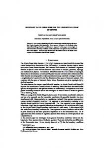
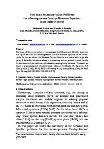
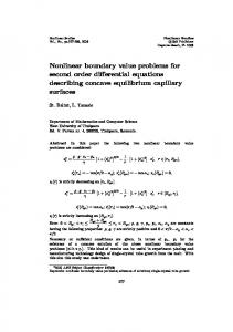
For special domains, it is possible to obtain precise regularity results. Let for example G have the form of steps as in the first two pictures below with angles π/2 or 3π/2 at every edge or the form of two beams, where one lies on the other as in the third picture. Note that the third polyhedron is not Lipschitz. The greatest edge angle is 3π/2, and we obtain min µk = 0.54448373.... Moreover for every vertex, there .. .. .. .. .. .. .. ..................................... . ... . . . . . . .... ....
.. .. . . ... ........... ... . . . .. .. ................................................ . . . . . . . .. .... .... . . . . .... .... . . . ..
.. .. .. ................................................... .. . ... ... ..... ... . . . . . . . .. ....................... .. ..... . . . .... ..... . . . . .... ..... .....
exists a circular cone with the same vertex and aperture 3π/2 which contains the polyhedron. The left polyhedron is even contained in a half-space bounded by a plane through an arbitrary of the vertices. Consequently, the smallest positive eigenvalue of the pencils Aj (λ) does not exceed the first eigenvalue for a circular cone with vertex 3π/2. A numerical calculation shows that this eigenvalue is greater than (3 min µk − 1)/2. This means that for β = 0 and δ = 0, the condition (iii) in Theorems 3.5 and 3.6 is stronger than the condition (ii) in the same theorems. Thus, we obtain (u, p) ∈ W 1,s (G)3 × Ls (G) (u, p) ∈ W 2,s (G)3 × W 1,s (G)
if f ∈ W −1,s (G), s < 2/(1 − min µk ) = 4.3905..., if f ∈ Ls (G), s < 2/(2 − min µk ) = 1.3740....
Here the condition on s is sharp. We give some comments concerning the examples in the introduction (the flow outside a regular polyhedron G). By Theorem 3.6, the regularity result (u, p) ∈ W 2,s × W 1,s in an arbitrary bounded subdomain of the complement of G holds if s < 2/(2 − µk ) and there are no eigenvalues of the pencils Aj (λ) in the strip −1/2 < Re λ < 2−3/s. Here, µk is the smallest positive √solution of the equation (3.13), where θk = θ is the edge angle in the exterior of G, sin θ is equal to − 23 2 if G is a regular tetrahedron √ or octahedron, −1 if G is a cube, − 52 5 if G is a regular dodecahedron, and −2/3 if G is a regular icosahedron. The smallest positive solutions of (3.13) are µk = 0.52033360... for the regular tetrahedron, µk = 0.54448373... for a cube, µk = 0.58489758... for the regular octahedron, µk = 0.60487306... for the regular dodecahedron, and µk = 0.68835272... for the regular icosahedron. In the case of a regular tetrahedron, cube, octahedron or dodecahedron, the inequality s < 2/(2 − µk ) implies 2 − 3/s < 3µk /2 − 1 < 0. Then the absence of eigenvalues of the pencil Aj (λ) in the strip −1/2 < Re λ < 2 − 3/s follows from [10, Th.5.5.6]. The exterior of a regular icosahedron is contained in a right circular cone with aperture less than 255◦ . Numerical results for right circular cones together with the monotonicity of the eigenvalues of the pencils Aj (λ) in the interval [−1/2, 1) show that also for this polyhedron, the strip −1/2 < Re λ < 3µk /2 − 1 is free of eigenvalues of the pencil Aj (λ). Thus, the above mentioned regularity result holds for all s < 2/(2 − µk ). This inequality cannot be weakened. The Neumann problem for the Navier-Stokes system. We consider a weak solution u ∈ W 1,2 (G)3 × L2 (G) of the Neumann problem −∆u + (u · ∇) u + ∇p = f, −∇u = 0 in G,
−pn + 2νεn (u) = 0 on Γj , j = 1, . . . , N.
For this problem it is known that the strip −1 ≤ Re λ ≤ 0 contains only the eigenvalues λ = 0 and λ = 1 of the operator pencils Aj (λ) (see [10, Th.6.3.2]) if G is a Lipschitz polyhedron. The numbers µk are the same as for the Dirichlet problem. Therefore, the following assertions are valid. ′
• If f ∈ (W 1,s (G)∗ )3 , s′ = s/(s − 1), 2 < s < 3, then (u, p) ∈ W 1,s (G)3 × Ls (G). • If f ∈ (W 1,2 (G)∗ )3 ∩ Ls (G)3 , 1 < s ≤ 4/3, then (u, p) ∈ W 2,s (G)3 × W 1,s (G).If the angles θk are less than 3 arccos 14 , then this result is true for 1 < s < 3/2. The mixed problem with Dirichlet and Neumann boundary conditions. We assume that on each face ∂u Γj either the Dirichlet condition u = 0 or the Neumann condition ∂n = 0 is given. If on both adjoining faces of the edge Mk the same boundary conditions are given, then µk > 1/2. If on one of the adjoining faces the Dirichlet condition and on the other face the Neumann condition is given, then µk > 1/4. This implies the following result. • If f ∈ (W 1,2 (G)∗ )3 ∩ Ls (G)3 , 1 < s ≤ 8/7, then every weak solution (u, p) belongs to W 2,s (G)3 × W 1,s (G). The mixed problem with boundary conditions (i)–(iii). Let (u, p) ∈ W 1,2 (G)3 × L2 (G) be a weak solution of the problem (1.2), (1.3), where g = 0, hj = 0, φj = 0 for j = 1, . . . , N , and dk ≤ 2 for all k (i.e., the Neumann condition does not appear in the boundary conditions). We assume that the Dirichlet condition is given on at least one of the adjoining faces of every edge. Then, by [10, Th.6.1.5], the strip −1 ≤ Re λ ≤ 0 is free of eigenvalues of the pencils Aj (λ). Furthermore, we have µk > 1/2 if the Dirichlet condition is given on both adjoining faces of the edge Mk . For the other indices k, we have µk > 1/4 and µk > 1/3 if θk < 23 π.
′
• If f ∈ (W 1,s (G)∗ )3 , 2 < s ≤ 8/3, then (u, p) ∈ W 1,s (G)3 × Ls (G). Suppose that θk < 32 π if the boundary condition (ii) or (iii) is given on one of the adjoining faces of the edge Mk . Then this result is even true for 2 < s ≤ 3. • If f ∈ (W 1,2 (G)∗ )3 ∩ Ls (G)3 , 1 < s ≤ 8/7, then (u, p) ∈ W 2,s (G)3 × W 1,s (G). Suppose that θk < 3 arccos 41 if the Dirichlet condition is given on both adjoining faces of Mk , θk < 23 arccos 41 if the boundary condition (ii) is given on one of the adjoining faces of Mk , and θk < 43 π if the boundary condition (iii) is given on one of the adjoining faces of Mk . Then the last result is true for 1 < s ≤ 3/2. Note that in the last case, we have µk > 2/3 for k = 1, . . . , m. Finally, we assume that the homogeneous Dirichlet condition u = 0 is given on the faces Γ1 , . . . , ΓN −1 , while the homogeneous boundary condition (iii) is given on ΓN . Let I be the set of all k such that ¯ N and I ′ = {1, . . . , m}\I. We suppose that the polyhedron G is convex and θk < π/2 for k ∈ I. Mk ⊂ Γ Then µk > 1 for all k, and the strip −1/2 ≤ Re λ ≤ 1 contains only the simple eigenvalue λ = 1 of the pencils Aj (λ) (see [10, Th.6.2.7]). If θk < 38 π for k ∈ I and θk < 43 π for k ∈ I ′ , then even µk > 4/3. This implies the following result. • Let f ∈ (W 1,2 (G)∗ )3 ∩ Ls (G)3 , 1 < s ≤ 2. Then any weak solution belongs to W 2,s (G)3 × W 1,s (G). If θk < 38 π for k ∈ I and θk < 34 π for k ∈ I ′ , then the result holds even for 1 < s < 3. Furthermore analogously to the Dirichlet problem, the following assertion holds. • Let f ∈ (W 1,2 (G)∗ )3 ∩ C −1,σ (G). Then for sufficiently small σ, we have (u, p) ∈ C 1,σ (G) × C 0,σ (G).
4
Existence of weak solutions in W 1,s(G) × Ls (G), s < 2
In Section 1 we proved the existence of weak solutions of the boundary value problem in W 1,2 (G)× L2 (G). Using the regularity result of Theorem 3.5, we obtain also the existence of weak solutions in W 1,s (G) × Ls (G) for sufficiently small s > 2. In this section, we will prove that weak solutions exist also in the space W 1,s (G)×Ls (G) with s < 2 provided the norms of the right-hand sides of (1.4), (1.5) in the corresponding Sobolev spaces are sufficiently small. Throughout this section, we suppose that the Dirichlet condition is given on at least one of the adjoining faces of every edge Mk .
4.1
Solvability of the linearized problem in a cone
1,s Let K be the same polyhedral cone as in Section 2.1. We consider weak solutions (u, p) ∈ Vβ,δ (G)3 × 0,s Vβ,δ (G) of the linear Stokes system in K with boundary conditions (i)–(iv) on the faces Γj . This means that (u, p) satisfies the equations Z 1,s′ (4.1) p ∇ · v dx = F (v) for all v ∈ V−β,−δ (K)3 , Sj v|Γj = 0, bK (u, v) − K
−∇ · u = g in K,
Sj u = hj on Γj , j = 1, . . . , N.
(4.2)
−1,s Here bK denotes the bilinear form (1.6), where G has to be replaced by K. We define the space Vβ,δ (K; S) ′
1,s as the set of all linear and continuous functionals on the space {v ∈ V−β,−δ (K)3 : Sj v|Γj = 0}, where ′ s = s/(s − 1). Furthermore, the pencils Ak (λ) for the edges Mk and A(λ) for the vertex of the cone K are defined as in Section 3.1. If the Dirichlet condition (i) is given on at least one of the adjoining faces of the edge Mk , then λ = 0 is not an eigenvalue of the pencil Ak (λ). (k) The following lemma is proved in [18] under the condition max(1 − Re λ1 , 0) < δk + 2/s < 1. Using the sharper estimates of Green’s matrix given in [17] for the case when λ = 0 is not an eigenvalue of the pencils Ak (λ), this theorem can be proved in the same way if (k)
(k)
1 − Re λ1 < δk + 2/s < 1 + Re λ1 for k = 1, . . . , N.
(4.3)
1−1/s,s
−1,s 0,s Lemma 4.1 Suppose that F ∈ Vβ,δ (K; S), g ∈ Vβ,δ (K), hj ∈ Vβ,δ (Γj ), there are no eigenvalues of the pencil A(λ) on the line Reλ = 1 − βj − 3/s, and the components of δ satisfy the inequalities (4.3). 1,s 0,s Then there exists a unique solution (u, p) ∈ Vβ,δ (K)3 × Vβ,δ (K) of problem (4.1), (4.2).
Moreover, the following regularity results hold analogously to [18, Le.4.4 and Th.4.4]. Lemma 4.2 1) Suppose that in addition to the assumptions of Lemma 4.1, we have F ∈ Vβ−1,t ′ ,δ ′ (K; S), 1−1/t,t
(k)
(k)
g ∈ Vβ0,t (Γj ), where 1 − Re λ1 < δk′ + 2/t < 1 + Re λ1 for k = 1, . . . , N and β ′ is ′ ,δ ′ (K), hj ∈ Vβ ′ ,δ ′ such that there are no eigenvalues of the pencil A(λ) in the closed strip between the lines Reλ = 1−β −3/s 1,s 0,s 0,t 3 and Reλ = 1 − β ′ − 3/t. Then the solution (u, p) ∈ Vβ,δ (K)3 × Vβ,δ (K) belongs to Vβ1,t ′ ,δ ′ (K) × Vβ ′ ,δ ′ (K). 2−1/t,t
2) Suppose that in addition to the assumptions of Lemma 4.1, g ∈ Vβ1,t ′ ,δ ′ (K), hj ∈ Vβ ′ ,δ ′ the functional F has the form Z N X Φj · v dx f · v dx + F (v) = K
(Γj ), and
j=1
1−1/t,t
with vector function f ∈ Vβ0,t (Γj ), where β ′ is such that there are no eigenvalues of ′ ,δ ′ (K), Φj ∈ Vβ ′ ,δ ′ the pencil A(λ) in the closed strip between the lines Reλ = 1 − β − 3/s and Reλ = 2 − β ′ − 3/t, and (k) (k) the components of δ ′ satisfy the inequalities 2 − Re λ1 < δk′ + 2/t < 2 + Re λ1 . Then the solution 1,s 0,s 1,t 3 (u, p) ∈ Vβ,δ (K)3 × Vβ,δ (K) belongs to Vβ2,t ′ ,δ ′ (K) × Vβ ′ ,δ ′ (K).
4.2
Solvability of the linearized problem in G
We consider the operator
1,s 0,s −1,s 0,s Vβ,δ (G)3 × Vβ,δ (G) ∋ (u, p) → (F, g, h) ∈ Vβ,δ (G; S) × Vβ,δ (G) ×
Y
1−1/s,s
Vβ,δ
(Γj )
(4.4)
j
−1,s of problem (1.9), (1.10) and denote this operator by As,β,δ . Here again Vβ,δ (G; S) is defined as the ′
1,s dual space of {v ∈ V−β,−δ (G)3 : Sj v|Γj = 0}. We show that this operator is Fredholm if there are no eigenvalues of the pencil Aj (λ) on the line Reλ = 1 − βj − 3/s, j = 1, . . . , d, and the components of δ satisfy the inequalities 1 − inf Re λ1 (ξ) < δk + 2/s < 1 + inf Re λ1 (ξ) (4.5) ξ∈Mk
ξ∈Mk
for k = 1, . . . , m. For this end, we construct a left and right regularizer for the operator As,β,δ . Lemma 4.3 Let U be a sufficiently small open subset of G and let ϕ be a smooth function with support in ¯ Suppose that there are no eigenvalues of the pencil Aj (λ) on the line Reλ = 1 − βj − 3/s, j = 1, . . . , d, U. and the components of δ satisfy (4.5). Then there exists an operator R continuously mapping the space Q 1−1/s,s 1,s 0,s −1,s 0,s (Γj ) with support in U¯ onto Vβ,δ (G)3 × Vβ,δ (G) such of all (F, g, h) ∈ Vβ,δ (G; S) × Vβ,δ (K) × j Vβ,δ ¯ that ϕAs,β,δ R(F, g, h) = ϕ(F, g, h) for all (F, g, h) with support in U and RAs,β,δ (u, p) = (u, p) for all (u, p) with support in U¯. P r o o f. Suppose first that U¯ contains the vertex x(1) of G. Then there exists a diffeomorphism κ mapping U onto a subset V of a polyhedral cone K with vertex at the origin such that κ(x(1) ) = 0 and the Jacobian matrix κ′ coincides with the identity matrix I at x(1) . We assume that the supports of u ¯ Then the coordinate change y = κ(x) transforms (1.9), (1.10) into and p are contained in U. Z 1,s′ ˜b(˜ ˜ v |det κ′ |−1 dy = F˜ (˜ u, v˜) − p˜ D˜ v ) for all v˜ ∈ Vβ,δ (K)3 , Sj v˜ = 0 on Γ◦j , (4.6) K
˜ u = g˜ in K, −D˜
Sj u˜ = ˜ hj on Γ◦j ,
(4.7)
˜ is a first order differential operator of the where u ˜ = u ◦ κ−1 , F˜ (˜ v ) = F (˜ v ◦ κ), Γ◦j are the faces of K, D form � ˜ u = D(y)∇y · u ˜, D˜
and ˜b is a bilinear form having the representation ˜b(˜ u, v˜) = 2ν
Z
3 X
K i,j=1
˜ · ∂yj v˜ dy. Bi,j (y) ∂yi u
Here D(y) and Bi,j (y) are quadratic matrices such that D(0) = I and 3 X
i,j=1
˜ · ∂yj v˜ = Bi,j (0) ∂yi u
3 X
εi,j (˜ u) εi,j (˜ v ).
i,j=1
Let ζ be an infinitely differentiable cut-off function on [0, ∞) equal to 1 in [0, 1) and to zero in (2, ∞). For arbitrary positive ǫ, we define ζǫ (y) = ζ(|y|/ǫ), Moreover, we put ζ0 = 0 and ηǫ = 1 − ζǫ for ǫ ≥ 0. We consider the operator Y 1−1/s,s 1,s 0,s ˜ ∈ V −1,s (K; S) × V 0,s (K) × Vβ,δ (Γ◦j ) (4.8) Vβ,δ (K)3 × Vβ,δ (K) ∋ (˜ u, p˜) → (F˜ , g˜, h) β,δ β,δ j
defined by � 1,s′ ˜ v |det κ′ |−1 + ηǫ ∇y · v˜ dy = F˜ (˜ v ) for all v˜ ∈ Vβ,δ (K)3 , Sj v˜ = 0 on Γ◦j , p˜ ζǫ D˜ K � ˜ j on Γ◦ , ˜ = g˜ in K, Sj u ˜=h − ζǫ D(y)∇y + ηǫ ∇y · u j
bǫ (˜ u, v˜) −
where
Z
bǫ (˜ u, v˜) = 2ν
Z
3 X
K i,j=1
� ˜ · ∂yj v˜ dy. ζǫ Bi,j (y) + ηǫ Bi,j (0) ∂yi u
We denote the operator (4.8) by A˜ǫ . According to Lemma 4.1, the operator A˜0 is an isomorhism. Since the norm of A˜0 − A˜ǫ is small for small ǫ, the operator A˜ǫ is an isomorphism if ǫ ≤ ǫ0 and ǫ0 is sufficiently small. We may assume that ζǫ = 1 on V for ǫ = ǫ0 . Then problem (4.6), (4.7) can be written as ¯ Let u, p˜) = (F˜ , g˜, ˜ h) if the supports of u ˜ and p˜ are contained in V. A˜ǫ0 (˜ u(x) = u ˜(κ(x)), p(x) = p˜(κ(x)) for x ∈ U,
˜ ˜ ˜, h). where (˜ u, p˜) = A˜−1 ǫ0 (F , g
(4.9)
1,s 0,s Outside U, let (u, p) be continuously extended to a vector function from Vβ,δ (G)3 × Vβ,δ (G). The so defined mapping (F, g, h) → (u, p) is denoted by R and has the desired properties. Suppose now that U¯ contains an edge point ξ ∈ M1 but no points of other edges and no vertices of G. Then again there exists a diffeomorphism mapping U onto a subset of a cone K. We assume that the point κ(ξ) lies on the edge M1◦ of K and coincides with the origin (in contrast to the first part of the proof, the vertex of the cone is not the origin). Let A˜ǫ be the same operator as above. Then there exist a number β0 and a tuple δ ′ , δ1′ = δ1 , such that A˜0 and for sufficiently small ǫ also A˜ǫ are isomorphisms Y 1−1/s,s 0,s −1,s 0,s 3 Vβ0 ,δ′ (Γ◦j ). Vβ1,s ′ (K) × Vβ ,δ ′ (K) → Vβ ,δ ′ (K; S) × Vβ ,δ ′ (K) × 0 ,δ 0 0 0 j
Since U¯ does not contain points of the edges Mk , k 6= 1, the vector function (4.9) can be continuously 1,s 0,s extended to a vector function from Vβ,δ (G)3 × Vβ,δ (G). The so defined mapping (F, g, h) → (u, p) defines the desired operator R. Analogously, the lemma can be proved for the case when U¯ contains no edge points of G. � Remark 4.1 Suppose that 2 − inf Re λ1 (ξ) < δk′ + 2/t < 2 + inf Re λ1 (ξ) for k = 1, . . . , m ξ∈Mk
ξ∈Mk
and there are no eigenvalues of the pencil Aj (λ) in the closed strip between the lines Reλ = 1 − βj − 3/s and Reλ = 2 − βj′ − 3/t. Then it follows from Lemma 4.2 that the operator R constructed in the proof of Lemma 4.3 continuously maps the subspace of all (F, g, h), where 1−1/s,s
0,s g ∈ Vβ,δ (G) ∩ Vβ1,t ′ ,δ ′ (G),
hj ∈ Vβ,δ
2−1/t,t
(Γj ) ∩ Vβ ′ ,δ′
(Γj )
−1,s and the functional F ∈ Vβ,δ (G; S) has the form
F (v) =
Z
G
f · v dx +
XZ j
Γj
Φj · v dx
1−1/t,t
3 with vector functions f ∈ Vβ0,t ′ ,δ ′ (G) , Φj ∈ Vβ ′ ,δ ′
(Γj )3 ,
1,t 3 into Vβ2,t ′ ,δ ′ (G) × Vβ ′ ,δ ′ (G).
Lemma 4.4 Suppose that there are no eigenvalues of the pencil Aj (λ) on the line Reλ = 1 − βj − 3/s, j = 1, . . . , d, and the components of δ satisfy (4.5). Then there exists a continuous operator Y 1−1/s,s 1,s 0,s −1,s 0,s Vβ,δ (Γj ) → Vβ,δ (G)3 × Vβ,δ (G) R : Vβ,δ (G; S) × Vβ,δ (K) × j
1,s 0,s −1,s such that RAs,β,δ − I and As,β,δ R − I are compact operators in Vβ,δ (G)3 × Vβ,δ (G) and Vβ,δ (G; S) × Q 1−1/s,s 0,s (Γj ), respectively. Vβ,δ (G) × j Vβ,δ
P r o o f. For the sake of brevity, we write A instead of As,β,δ . Let {Uj } be a sufficiently fine open covering of G, and let ϕj , ψj be infinitely differentiable functions such that X ϕj = 1. supp ϕj ⊂ supp ψj ⊂ Uj , ϕj ψj = ϕj , and j
For every j, there exists an operator Rj having the properties of Lemma 4.2 for U = Uj ∩ G. We consider the operator R defined by X ϕj Rj ψj (F, g, h). R (F, g, h) = j
Obviously, R A(u, p) =
X j
X � ϕj Rj [A, ψj ] (u, p), ϕj Rj Aψj (u, p) − [A, ψj ] (u, p) = (u, p) − j
where [A, ψj ] is the commutator of A and ψj . Here, the mapping (u, p) → [A, ψj ] (u, p) is continuous 1,s 0,s from Vβ,δ (G)3 × Vβ,δ (G) into the set of all (F, g, h), where g ∈ Vβ1,s ′ ,δ ′ (G), h = 0, and F is a functional of the form Z XZ 1−1/s,s 3 F (v) = f · v dx + Φj · v dx, where f ∈ Vβ0,s (Γj )3 , ′ ,δ ′ (G) , Φj ∈ Vβ ′ ,δ ′ G
j
Γj
with arbitrary β ′ ≥ β, δ ′ ≥ δ. We can choose β ′ and δ ′ such that βj ≤ βj′ < βj + 1 for j = 1, . . . , d, δk ≤ δk′ < δk + 1 for k = 1, . . . , m, and β ′ , δ ′ satisfy the conditions of Remark 4.1 with t = s. Then 1,s 0,s 1,s 3 the mapping (u, p) → Rj [A, ψj ] (u, p) is continuous from Vβ,δ (G)3 × Vβ,δ (G) into Vβ2,s ′ ,δ ′ (G) × Vβ ′ ,δ ′ (G). 1,s 0,s 3 ′ ′ Since the last space is compactly imbedded into Vβ,δ (G) × Vβ,δ (G) for βj < βj + 1, δk < δk + 1 (cf. [9, Le.6.2.1]), it follows that RA − I is compact. Analogously, the compactness of AR − I holds. � From Lemma 4.4 it follows that the operator As,β,δ is Fredholm under the conditions of this lemma. Using Theorem 1.1 and Lemma 4.2, we can prove the following theorem on the existence of unique solutions.
1−1/s,s
−1,s 0,s Theorem 4.1 Let F ∈ Vβ,δ (G; S), g ∈ Vβ,δ (G), and hj ∈ Vβ,δ (Γj )3−dj . We suppose that the components of δ satisfy condition (4.3) and that there are no eigenvalues of the pencils Aj (λ) in the closed strip between the lines Re λ = −1/2 and Re λ = 1 − β − 3/s. In the case when dj ∈ {0, 2} for all j, we assume in addition that g and hj satisfy condition (1.11). Then there exists a solution (u, p) ∈ 1,s 0,s 1,s′ Vβ,δ (G)3 × Vβ,δ (G) of problem (1.9), (1.10). (Here V has to be replaced by the set of all v ∈ V−β,−δ (G) satisfying Sj v = 0 on Γj .) The vector function u is unique, p is unique if dj 6∈ {0, 2} for at least one j, p is unique up to a constant if dj ∈ {0, 2} for all j.
P r o o f. First note that in the case when dj ∈ {0, 2} for all j, the spectra both of Aj (λ) and Ak (λ) contain the eigenvalue λ = 1. An eigenvector corresponding to this eigenvalue is (U, P ) = (0, 1). Furthermore, the spectra of the pencils Aj (λ) contain the eigenvalue λ = −2. Therefore from the conditions of the lemma on β and δ it follows in particular that 0 < βj + 3/s < 3 and 0 < δk + 2/s < 2. 0,s 0,s Then L∞ (G) ⊂ Vβ,δ (G) ⊂ L1 (G). In particular, any constant belongs to the space Vβ,δ (G), and the 1−1/s,s
0,s integrals in (1.11) exist for g ∈ Vβ,δ (G), hj ∈ Vβ,δ (Γj )3−dj . 1,s 0,s We prove the uniqueness of u and p. Let (u, p) ∈ Vβ,δ (G)3 × Vβ,δ (G) be a solution of problem (1.9), 1,2 (1.10) with F = 0, g = 0, hj = 0. Then according to Lemma 4.2, we have u ∈ V0,0 (G)3 ⊂ W 1,2 (G)3 and p ∈ L2 (G). From Theorem 1.1 it follows that u = 0 and p is constant, p = 0 if dj ∈ {1, 3} for at least one j. We prove the existence of solutions for the case when dj ∈ {0, 2} for all j. Due to Lemma 4.4 and the R 1,s 0,s uniqueness of the solution, every solution (u, p) ∈ Vβ,δ (G)3 × Vβ,δ (G) of problem (1.9), (1.10), G p dx = 1, satisfies the inequality � � X (4.10) khj kV 1−1/s,s (Γj ) kukV 1,s (G)3 + kpkV 0,s (G) ≤ c kF kV −1,s (G;S)) + kgkV 0,s (G) + β,δ
β,δ
β,δ
β,δ
β,δ
j
1−1/s,s
−1,s 0,s with a constant c independent of u and p. Let F ∈ Vβ,δ (G; S), g ∈ Vβ,δ (G) and hj ∈ Vβ,δ (Γj )3−dj −1,s 0,s satisfying (1.11) be given. Then there exist sequences {F (n) } ⊂ V ∗ ∩Vβ,δ (G; S), {g (n) } ⊂ L2 (G)∩Vβ,δ (G) 1−1/s,s
(n)
(Γj )3−dj converging to F , g, and hj , respectively. From (1.11) it and {hj } ⊂ W 1/2,2 (Γj )3−dj ∩ Vβ,δ follows that the sequences of the numbers Z X Z X Z (n) (n) hj dx hj · n dx + g (n) dx + an = G
j: dj =0
Γj
j: dj =2
Γj
converges to zero. Therefore, the sequence of the functions g˜(n) = g (n) −
1 |G|
an converges also to g.
(n) hj
satisfy condition (1.11). By Theorem 1.1, there exist solutions (u(n) , p(n) ) ∈ (n) R W 1,2 (G)3 × L2 (G) of problem (1.9), (1.10) with right-hand sides F (n) , g˜(n) and hj , G p(n) dx = 0. 1,2 From Lemma 4.2 and from the imbedding W 1,2 (G) ⊂ V0,ε (G) with arbitrary positive ε it follows that 1,s 0,s (n) (n) 3 (u , p ) ∈ Vβ,δ (G) × Vβ,δ (G). Due to (4.10), the vector functions (u(n) , p(n) ) form a Cauchy sequence 1,s 0,s in Vβ,δ (G)3 × Vβ,δ (G). The limit of this sequence solves problem (1.9), (1.10). The proof of the existence of solutions in the case when dj ∈ {1, 3} for at least one j proceeds analogously. � (n)
Moreover, g˜
4.3
and
Solvability of the nonlinear problem
1,s We consider the nonlinear problem (1.2), (1.3). For the proof of the existence of solutions in Vβ,δ (G)3 × 0,s Vβ,δ (G), we have to have to show inequalities analogous to (1.13), (1.14) for the operator 1,s −1,s Vβ,δ (G)3 ∋ u → Qu = (u · ∇)u ∈ Vβ,δ (G; S).
Lemma 4.5 Suppose that s > 3/2, βj + 3/s ≤ 2 for j = 1, . . . , N , and δk + 3/s ≤ 2 for k = 1, . . . , m. Then ku ∂xj vkV −1,s (G)3 ≤ c kukV 1,s (G) kvkV 1,s (G) β,δ
for all u, v ∈
1,s Vβ,δ (G),
j = 1, 2, 3.
β,δ
β,δ
P r o o f. Let t be a real number such that t ≥ 3, t ≥ s,
3 3 3 −1≤ 1. By H¨ olders’s inequality, we have
ku∂xj vkV 0,q ′
β+β ,δ+δ′
(G)
≤ c kukV 0,t k∂xj vkV 0,s (G) ′ ′ (G) β,δ
β ,δ
1,s 0,q −1,s for arbitrary u, v ∈ Vβ,δ (G). Using the continuity of the imbedding Vβ+β (G) which ′ ,δ+δ ′ (G) ⊂ Vβ,δ follows from Corollary 2.2, we obtain the desired inequality. � 1,s As a consequence of Lemma 4.5, the following inequalities hold for arbitrary u, v ∈ Vβ,δ (G)3 :
kQukV −1,s (G;S) ≤ c kuk2V 1,s (G)3 , β,δ
(4.11)
β,δ
�
kQu − QvkV −1,s (G;S) ≤ c kukV 1,s (G)3 + kvkV 1,s (G)3 ku − vkV 1,s (G))3 . β,δ
β,δ
β,δ
β,δ
(4.12)
Using these estimates, the following theorem can be proved analogously to Theorem 1.2. Theorem 4.2 Let the conditions of Theorem 4.1 on F , g hj , β and δ be satisfied. In addition, we assume that s > 3/2, βj + 3/s ≤ 2, δk + 3/s ≤ 2 and that X khj kV 1−1/s,s (Γj )3−dj kF kV −1,s (G;S) + kgkV 0,s (G) + β,δ
β,δ
j
β,δ
1,s 0,s is sufficiently small. Then there exists a solution (u, p) ∈ Vβ,δ (G)3 × Vβ,δ (G) of problem (1.4), (1.5), ′
1,s where V has to be replaced by the set of all v ∈ V−β,−δ (G)3 such that Sj v = 0 on Γj , j = 1, . . . , N . The function u is unique on the set of all functions with norm less than a certain positive ε, p is unique if dj ∈ {1, 3} for at least one j, otherwise p is unique up to a constant.
1,s 0,s P r o o f. Let (u(0) , p(0) ) ∈ Vβ,δ (G)3 × Vβ,δ (G). By Theorem 4.1, the norm of u(0) can be assumed to be small. Obviously, (u, p) is a solution of problem (1.4), (1.5) if and only if (w, q) = (u − u(0) , p − p(0) ) is a solution of the problem Z Z 1,s′ (G)3 , Sj v|Γj = 0, q ∇ · v dx = − Q(w + u(0) ) · v dx for all v ∈ v ∈ V−β,−δ b(w, v) − G
G
∇ · w = 0 in G,
Sj u = 0 on Γj , j = 1, . . . , N.
This problem can be written as (w, q) = −AQ(w + u(0) ) where A is the inverse to the operator F → As,β,δ (F, 0, 0) considered in the preceding subsection. Due to 1,s 0,s (4.12), the operator (w, q) → −AQ(w + u(0) ) is contractive on the set of all (w, q) ∈ Vβ,δ (G)3 × Vβ,δ (G) (0) with norm ≤ ε if ε and the norm of u are sufficiently small. Hence this operator has a fixed point. This proves the theorem. � Finally, we give a result in nonweighted Sobolev spaces which follows immediately from the last theorem. Let G be a polyhedron. We assume that on every face Γj , one of the boundary conditions (i)–(iii) is given, that the Dirichlet condition is given on at least one of the adjoining faces of every edge Mk ,
and that θk ≤ 3π/2 if the boundary conditions (ii) or (iii) are given on one of the adjoining faces of Mk . Here, θk denotes again the angle at the edge Mk . Then the problem Z X 3
∂u · v dx − uj b(u, v) + ∂xj G j=1 −∇ · u = 0 in G,
Z
G
′
p ∇ · v dx = F (v) for all v ∈ W 1,s (G)3 , Sj v = 0 on Γj ,
Sj u = 0 on Γj , j = 1, . . . , N,
with F ∈ W −1,s (G; S), 3/2 < s < 3, has a solution (u, p) ∈ W 1,s (G)3 × Ls (G) if the norm of F is sufficiently small. For the proof it suffices to note that the strip −1 ≤ Re λ ≤ 0 does not contain eigenvalues of the pencils (k) Aj (λ) and that Re λ1 ≥ 1/3 for k = 1, . . . , m. Therefore, the conditions of Theorem 4.2 are satisfied for β = 0, δ = 0, 3/2 < s < 3.
References [1] Dauge, M., Stationary Stokes and Navier-Stokes systems on two- and three-dimensional domains with corners. Part 1: Linearized equations, SIAM J. Math. Anal. 20 (1989) 74-97. [2] Deuring, P., von Wahl, W., Strong solutions of the Navier-Stokes system in Lipschitz bounded domains, Math. Nachr. 171 (1995) 111-148. [3] Dindos, M., Mitrea, M., The stationary Navier-Stokes system in nonsmooth manifolds: The Poisson problem in Lipschitz and C 1 domains, Arch. Ration. Mech. Anal. 174 (2004) 1, 1-47. [4] Ebmeyer, C., Frehse, J., Steady Navier-Stokes equations with mixed boundary value conditions in three-dimensional Lipschitzian domains, Math. Ann. 319 (2001) 349-381. [5] Girault, V., Raviart, P.-A., Finite element methods for Navier-Stokes equations, SpringerVerlag, Berlin-Heidelberg-New York-Tokyo 1986. [6] Kalex, H.-U., On the flow of a temperature dependent Bingham fluid in non-smooth bounded twodimensional domains, Z. Anal. Anwendungen 11 (1992) 4, 509-530. [7] Kellogg, R. B., Osborn, J., A regularity result for the Stokes problem in a convex polygon, J. Funct. Anal. 21 (1976) 397-431. [8] Kondrat’ev, V. A., Asymptotic of solutions of the Navier-Stokes equation near an angular point of the boundary, J. Appl. Math. Mech. 31 (1967) 125-129. [9] Kozlov, V. A., Maz’ya, V. G., Rossmann, J., Elliptic boundary value problems in domains with point singularities, Mathematical Surveys and Monographs 52, Amer. Math. Soc., Providence, Rhode Island 1997. [10] Kozlov, V. A., Maz’ya, V. G., Rossmann, J., Spectral problems associated with corner singularities of solutions to elliptic equations, Mathematical Surveys and Monographs 85, Amer. Math. Soc., Providence, Rhode Island 2001. [11] Kozlov, V. A., Maz’ya, V. G., Schwab, C., On singularities of solutions to the Dirichlet problem of hydrodynamics near the vertex of a cone, J. Reine Angew. Math. 456 (1994) 65-97. [12] Ladyzhenskaya, O. A., Funktionalanalytische Untersuchungen der Navier-Stokesschen Gleichungen, Akademie-Verlag Berlin 1965. [13] Maz’ya, V. G., Plamenevski˘ı, B. A., The first boundary value problem for classical equations of mathematical physics in domains with piecewise smooth boundaries, Part 1: Zeitschr. Anal. Anw. 2 (4) 1983, 335-359, Part 2: Zeitschr. Anal. Anw. 2 (6) 1983, 523-551.
[14] Maz’ya, V. G., Plamenevski˘ı, B. A., Stupelis, L., The three-dimensional problem of steadystate motion of a fluid with a free surface, Amer. Math. Soc. Transl. 123 (1984) 171-268. ¨ [15] Maz’ya, V. G., Rossmann, J., Uber die Asymptotik der L¨ osungen elliptischer Randwertaufgaben in der Umgebung von Kanten, Math. Nachr. 138 (1988) 27-53. [16] Maz’ya, V. G., Rossmann, J., On the Agmon-Miranda maximum principle for solutions of elliptic equations in polyhedral and polygonal domains, Ann. Global Anal. Geom. 9 (1991) 3, 253-303. [17] Maz’ya, V. G., Rossmann, J., Point estimates of Green’s matrix for a mixed boundary value problem to the Stokes system in a polyhedral cone, to appear in Math. Nachr., Preprint mathph/0412068 in www.arxiv.org. [18] Maz’ya, V. G., Rossmann, J., Lp estimates of solutions to mixed boundary value problems for the Stokes system in polyhedral domains, to appear., Preprint math-ph/0412073 in www.arxiv.org. [19] Maz’ya, V. G., Rossmann, J., Schauder estimates for solutions to mixed boundary value problems for the Stokes system in polyhedral domains, to appear in Math. Methods Appl. Sci. [20] Nicaise, S., Regularity of the solutions of elliptic systems in polyhedral domains, Bull. Belg. Math. Soc. 4 (1997) 411-429. [21] Orlt, M., S¨ andig, A.-M., Regularity of viscous Navier-Stokes flows in nonsmooth domains, Boundary Value Problems and Integral Equations in Nonsmooth Domains, Lecture Notes in Pure and Appl. Math. 167 (1993) 185-201. [22] Rossmann, J., On two classes of weighted Sobolev-Slobodetski˘ı spaces in a dihedral angle, Partial Differential Equations, Banach Center Publications 27 (1992) 399-424. [23] Solonnikov, V. A., Solvability of a three-dimensional boundary value problem with a free surface for the stationary Navier-Stokes system, Partial Differential Equations, Banach Center Publications, Vol. 10, Warsaw 1983, 361-403. [24] Solonnikov, V. A., Scadilov, V. E., On a boundary value problem for a stationary system of Navier-Stokes equations, Trudy Math. Steklov 125 (1973) 196-210. [25] Temam, R., Navier-Stokes equations, theory and numerical analysis, North-Holland, Amsterdam 1977