finite elements for the solution of nonlinear solid mechanics prob- lems. ...... Financial support from the Spanish Ministry for Education and Science under.
Mixed Stabilized Finite Element Methods in Nonlinear Solid Mechanics. Part I: Formulation M. Cervera, M. Chiumenti and R. Codina International Center for Numerical Methods in Engineering (CIMNE) Technical University of Catalonia (UPC) Edificio C1, Campus Norte, Jordi Girona 1-3, 08034 Barcelona, Spain.
K�������: mixed finite element interpolations, stabilization methods, algebraic sub-grid scales, orthogonal sub-grid scales, nonlinear solid mechanics. Abstract This paper exploits the concept of stabilized finite element methods to formulate stable mixed stress/displacement and strain/displacement finite elements for the solution of nonlinear solid mechanics problems. The different assumptions and approximations used to derive the methods are exposed. The proposed procedure is very general, applicable to 2D and 3D problems and independent of the constitutive equation considered. Implementation and computational aspects are also discussed, showing that a robust application of the proposed formulation is feasible. Numerical examples show that the results obtained compare favourably with those obtained with the corresponding irreducible formulation.
1
1
Introduction
The term mixed methods has been used in the finite element method literature since the mid 1960’s to denote formulations in which both the displacement and stress fields are approximated as primary variables [1]. Despite their doubtless interest from the theoretical point of view, the practical application of mixed methods is greatly outnumbered by the implementation of irreducible methods, in which only the displacement field is considered primary variable of the problem and the stress field is obtained a posteriori by differentiation. However, there are several fields of application in computational solid mechanics in which mixed methods are well established and regularly used in practice. For instance, it is well known that standard irreducible low order finite elements perform miserably in nearly incompressible situations, producing solutions which are almost completely locked by the incompressibility constraint. Remedies for this undesirable behaviour have been actively sought for decades. In fact, the purely incompressible problem (Stokes problem) does not admit an irreducible formulation and, consequently, a mixed framework in terms of displacements and pressure is necessary for these situations. Over the years, and particularly in the 1990’s, different strategies were proposed and tested to reduce or avoid volumetric locking and pressure oscillations in finite element solutions with different degrees of success ([2, 3, 4, 5, 6, 7, 8, 9, 10, 11, 12, 13, 14]). Many of these methods, while resembling displacement methods, have been shown to be equivalent to more general mixed methods. Another common application of mixed methods is plate bending problems and other fourth order problems ([15, 5, 16, 17]). Here, the motivation is the avoidance of C 1 -continuity in the definition of the interpolation functions, required if the primal variational functional is used. As an alternative, the mixed functional only involves second derivatives and, after integration by parts, C 0 -continuous element may be used. Another alternative is the use of non-conforming elements. The reasons for the limited popularity of mixed methods in computational solid mechanics are twofold: computational cost and lack of stability [18, 19, 20]. On one hand, because mixed methods approximate both displacements and stresses simultaneously, the corresponding discrete systems of equations involve many more degrees of freedom than the corresponding irreducible formulations. Concurrently, the mixed system of equations 2
is very often indefinite, which makes most of the direct and iterative solution methods inapplicable. These difficulties may be avoided with a suitable implementation. On the other hand, many choices of the individual interpolation fields for the mixed problem yield meaningless, not stable, results. This is due to the strictness of the inf-sup condition [19] when the standard Galerkin finite element method is applied straightforwardly to mixed elements, as it imposes severe restrictions on the compatibility of the interpolations used for the displacement and the stress fields. This difficulty, if not circumvented, is severely restrictive (see [21] and [22, 23] for the analysis of admissible elements in linear elasticity). In parallel, mixed methods have also been the focus of attention in computational fluid dynamics. In [24] and [25], the variational multiscale (VMS) formulation was proposed as a new way of circumventing the difficulties posed by the inf-sup condition. In the case of incompressible problems, the reasoning behind was not new, as it consisted of modifying the discrete variational form to attain control on the pressure field. The result was the possibility of using equal order interpolations for displacements and pressures and to construct stable low order elements. Since then, the sub-grid concept underlying the VMS approach has been extensively and fruitfully used in fluid dynamics. In [26] and [27], the concept of orthogonal subscale stabilization (OSS) was introduced, which leads to well sustained and better performing stabilization procedures. The analysis of the formulation can be found in [28] for the linearized incompressible Navier-Stokes equations and, in subjects closer to the topic of this paper, in [29] for the stress-displacement-pressure formulation of the Stokes problem (equivalent to the linear elastic incompressible problem) and in [30] for Darcy’s problem. In previous works, the authors have applied stabilized mixed displacement/pressure methods (see [31, 32, 33, 34, 35] and [36]) to the solution of incompressible J2 -plasticity and damage problems with strain localization using linear/linear simplicial elements in 2D and 3D. These procedures lead to a discrete problem which is fully stable, free of pressure oscillations and volumetric locking and, thus, results obtained are practically mesh independent. This translates in the achievement of two important goals: (a) the position and orientation of the localization band is independent of the directional bias of the finite element mesh and (b) the global post-peak load-deflection curves are independent of the size of the elements in the localization band. Similar ideas have been used in [37, 38] and [39]. In the present work we extent this approach in order to derive stable 3
mixed stress-displacement and strain-displacement formulations using linear/linear interpolations in triangular elements and bilinear/bilinear interpolations in quadrilateral elements. Our goal is to solve the problem of strain localization in the context of compressible nonlinear solid mechanics. The basic motivation for this work is to prove that the difficulties encountered when solving solid mechanics problems involving the creation and propagation of strain localization bands using standard elements and local constitutive models are due to the approximation error inherent to the spatial discretization, as well as to the poor stability in the stresses and/or strains. When using the basic, irreducible, formulation of the problem, the stresses (or strains), which are the variables of most interest for the satisfaction of the highly nonlinear constitutive behaviour, are not the fundamental unknowns of the problem and they are obtained by differentiation of the displacement field, a process which entails an important loss of accuracy, particularly where strong displacement gradients occur. The local approximation error committed makes propagation of the localization bands strongly dependent on the finite element mesh used. Contrariwise, when using a mixed formulation in which the stress (or the strain) field is selected as primary variable, together with the displacement field, the added accuracy and stability achieved are enough to overcome the mesh dependency problem satisfactorily. The outline of the present paper is as follows. In the next section the mixed stress/displacement (σ/u) finite element formulation for linear elasticity is summarized. The sub-grid scale approach is outlined and two stabilized formulations are derived. Results concerning stability and convergence of these schemes are discussed. In Section 3 the stabilization is extended to nonlinear problems, proposing both stress-displacement and a strain-displacement formulations. The later can be considered more suitable for the implementation of nonlinear constitutive models such as plasticity and damage models. Implementation and computational aspects are discussed next. Finally, some numerical benchmarks and examples are presented to assess the present formulation and to compare its performance with the standard irreducible elements. The problem of strain localization is discussed in a companion paper.
4
2 2.1
Mixed stabilized stress—displacement formulation in linear elasticity Continuous problem
The formulation of the solid mechanics problem can be written considering the stress as an independent unknown, additional to the displacement field. In this case, the strong form of the continuum problem can be stated as: given a field of prescribed body forces f and a constant constitutive tensor C, find the displacement field u and the stress field σ such that: −σ + C : ∇s u = 0 ∇·σ+f = 0
in Ω in Ω
(1a) (1b)
where Ω is the open and bounded domain of Rndim occupied by the solid in a space of ndim dimensions. Equations (1a)-(1b) are subjected to appropriate Dirichlet and Neumann boundary conditions. In the following, we will assume these, without loss of generality, in the form of prescribed displacements u = 0 on ∂Ωu , and prescribed tractions t on ∂Ωt , respectively, being ∂Ωu and ∂Ωt a partition of ∂Ω. Multiplying by the test functions and integrating by parts the second equation, the associated weak form of the problem (1a)-(1b), can be stated as: � � − τ , C−1 : σ + (τ ,∇s u) = 0 ∀τ (2a) � � s (∇ v, σ) = (v, f ) + v, t ∂Ωt ∀v (2b)
where v ∈ V and τ ∈ T are the test functions of the displacement and stress fields, respectively, and (·, ·) denotes the inner product in L2 (Ω), the space of square integrable functions in Ω. Hereafter, orthogonality will be understood with respect to this product. Likewise, (v, ¯t)∂Ωt denotes the integral �of v �and ¯t over ∂Ωt . For the sake of shortness, we will write F(v) = (v, f) + v, t ∂Ωt in the following. Equations (2a)-(2b) can be understood as the stationary conditions of the classical Hellinger-Reissner functional. The space of stresses T consists of symmetric tensor whose components are in L2 (Ω). If the weak form is written as indicated in (2a), the displacements and their test functions have to have components in H 1 (Ω) (they and 5
their derivatives have to be in L2 (Ω)) and must vanish on ∂Ωu . This defines the space of displacements V. However, it is also possible to integrate the second term in (2a) by parts, obtaining (τ , ∇s u) = −(∇·τ , u), and similarly for the left-hand-side of (2b). In this case, the components of the stresses have to have also the divergence in L2 (Ω), but the components of the displacement need to be only in L2 (Ω), not H 1 (Ω). Similarly to Darcy’s problem, there are two possible functional settings for the linear elastic problem written in mixed form (see [30]). This is not essential for our discussion, although it has some implications in the treatment of boundary conditions on which we will not enter.
2.2
Galerkin finite element approximation
Let us now define the discrete Galerkin finite element counterpart problem as: � � ∀τ h (3a) − τ h , C−1 : σ h + (τ h ,∇s uh ) = 0 s (∇ vh , σ h ) = F(vh ) ∀vh (3b) where uh , vh ∈ Vh and σ h , τ h ∈ Th are the discrete displacement and stress fields and their test functions, defined onto the finite element spaces Vh and Th , respectively. Note that the resulting system of equations is symmetric but non-definite. In all what follows, we will be interested in continuous finite element spaces Vh and Th and, more specifically, in equal interpolation for stresses and displacements. Therefore, we may replace (τ h , ∇s vh ) by −(∇ · τ h , vh ), for all vh ∈ Vh and τ h ∈ Th . As it is well known, the stability of the discrete formulation depends on appropriate compatibility restrictions on the choice of the finite element spaces Vh and Th , as stated by the inf-sup condition [19]. According to this, standard Galerkin mixed elements with continuous equal order linear/linear interpolation for both fields are not stable. Lack of stability shows as uncontrollable oscillations in the displacement field that entirely pollute the solution. Fortunately, the strictness of the inf-sup condition can be avoided by modifying the discrete variational form, for instance, by means of introducing appropriate numerical techniques that can provide the necessary stability to the desired choice of interpolation spaces. The objective of this work is precisely to present stabilization methods which allow the use of equal order continuous interpolations for displacements and stresses. 6
2.3 2.3.1
Stabilized finite element methods Scale splitting
The basic idea of the sub-grid scale approach [24] is to consider that the continuum unknowns can be split in two components, one coarse and a finer one, corresponding to different scales or levels of resolution. The solution of the continuum problem contains components from both scales. For the solution of the discrete problem to be stable it is necessary to, somehow, include the effect of both scales in the approximation. The coarse scale can be appropriately solved by a standard finite element interpolation, which however cannot solve the finer scale. Nevertheless, the effect of this finer scale can be included, at least locally, to enhance the stability of the displacement in the mixed formulation. To this end, the stress and the displacement fields of the mixed problem will be approximated as �, σ = σh + σ
� u = uh + u
(4)
where σ h ∈ Th and uh ∈ Vh are the components of the stresses and the � are � ∈ T� and u �∈V displacements on the (coarse) finite element scale and σ the enhancement of the stresses and the displacements corresponding to the (finer) sub-grid scales. Let us also consider the corresponding test functions � This approximation extends the stress solution space � ∈ V. τ� ∈ T� and v � Each to T � Th ⊕ T� , and the displacement solution space to V � Vh ⊕ V. particular stabilized finite element method is defined according to the way � are chosen. In particular, the Galerkin method in which spaces T� and V � = {0}. corresponds to taking T� = {0}, V As it has been mentioned, in what follows we will consider continuous finite element interpolations. Likewise, we will assume that the subscales vanish on the interelement boundaries. When more general situations are considered, additional terms involving interelement boundary integrals need to be added (see [30, 40]). Introducing the splitting, the problem corresponding to (2a)-(2b) is: � � � � � + (τ h ,∇s uh ) − (∇ · τ h ,� u) = 0 ∀τ h (5a) − τ h , C−1 : σ h − τ h , C−1 : σ � � � � � + (� �) = 0 ∀� − τ� , C−1 : σ h − τ� , C−1 : σ τ ,∇s uh ) + (� τ ,∇s u τ (5b) s s � ) = F(vh ) ∀vh (5c) (∇ vh , σ h ) + (∇ vh , σ � ) = F(� − (� v, ∇ · σ h ) − (� v, ∇ · σ v) ∀� v (5d) 7
where some terms have been integrated by parts and we have assumed that � and v � vanish on the boundary. In the following, the fact that the discrete u variational equations need to hold for all test functions will be omitted. Due to the approximation used, (4), and the linear independence of τ h and τ� , now the continuum equation (2a) unfolds in two discrete equations, (5a) and (5b), one related to each scale considered. The same comment is applicable to the displacement splitting. Equations (5a) and (5c) are defined in the finite element spaces Th and Vh , respectively. The first �one enforces �the � − constitutive equation including a stabilization term S1 = − τ h , C−1 : σ (∇ · τ h ,� u) depending on the sub-grid stresses and displacements. The second one solves the balance of momentum including a stabilization term S2 = � ) depending on the sub-grid stresses σ �. (∇s vh , σ Let us define the residuals of the finite element components as rσ,h = C−1 : σ h − ∇s uh ru,h = f + ∇ · σ h
These allow us to write (5b) and (5d) as � � � + (� � ) = (� − τ� , C−1 : σ τ ,∇s u τ , rσ,h ) � ) = (� − (� v, ∇ · σ v, ru,h )
(6a) (6b)
(7a) (7b)
These equations are the projections of the finite element residuals onto the space of sub-scales, which cannot be resolved by the finite element mesh. Therefore, to proceed it is necessary to provide an approximate closed form �u are the projections onto T� and V, � respectively, �σ and P solution to them. If P note first that we may write (7a) and (7b) as �σ (−C−1 : σ �σ (rσ,h ) � + ∇s u �) = P P �u (ru,h ) �) = P P�u (−∇ · σ
(8a) (8b)
and therefore the problem is to approximate the operators on the left-handside of these equations. The way we motivate such an approximation is by using an approximate Fourier analysis of the problem. Using exactly the same � and u � may be approximated procedure as in [41], it can be shown that σ within each element by �σ (rσ,h ) = τ σ P �σ (C : ∇s uh − σ h ) � = −τ σ C : P σ �u (ru,h ) = τ u P �u (f + ∇ · σ h ) � = τ uP u 8
(9a) (9b)
where the so called stabilization parameters τ σ and τ u can be computed as τ σ = cσ
h , L0
τ u = cu
L0 h Cmin
(10)
and where cσ and cu are algorithmic constants, L0 is a characteristic length of the computational domain, h is the element size and Cmin > 0 is the smallest eigenvalue of C (see below). As shown in [30], this is the choice of the parameters that yields best order of convergence for equal order of interpolation of stresses and displacements. In the following, and for the sake of clarity, we will consider the mesh quasi-uniform, so that a unique h can be defined for all the mesh, and thus τ σ and τ u will be constant. In general situations, it is understood that these parameters have to be evaluated elementwise. The methods we wish to consider are completely defined up to the choice �u . Two possible options are described next. �σ and P of the projections P 2.3.2
Residual based algebraic subgrid scale method
�σ and P�u as the identity when applied to the The simplest choice is to take P residuals in (9a) and (9b). In fact, one may also think that the projection is scaled by the stabilization parameters given by (10), which act as upscaling of the residuals onto the finite element mesh. This is what is called algebraic subgrid scale (ASGS) method in [30], for example. If the subscales resulting from these equations are then inserted into (5a) and (5c) one gets � � − (1 − τ σ ) τ h , C−1 : σ h + (1 − τ σ ) (τ h , ∇s uh ) − τ u (∇ · τ h , ∇ · σ h ) = τ u (∇ · τ h , f) (11a) (1 − τ σ ) (∇s vh , σ h ) + τ σ (∇s vh , C : ∇s uh ) = F(vh ) (11b) Note that the resulting system of equations is symmetric. Particularly interesting is the case τ u = 0. In this situation, (11a) represents a projection onto the discrete finite element space that can be written as σ h = Ph (C : ∇s uh ) (12) and, therefore, the discrete balance equation (11b) takes the form: (1 − τ σ ) (∇s vh ,Ph (C : ∇s uh )) + τ σ (∇s vh , C : ∇s uh ) = (vh , f) Thus, for τ u = 0 the method we propose can be rewritten as σ stab = (1 − τ σ ) Ph (C : ∇s uh ) + τ σ (C : ∇s uh ) (∇s vh , σ stab ) = F(vh ) 9
(13a) (13b)
This compact form of writing the problem is only possible when τ u = 0. Otherwise, (11a)-(11b) have to be kept as such. Some remarks are in order: 1. The stabilization term S2 in (5c) is computed in an element by element manner and within each element. Its magnitude depends on the difference between the continuous (projected) stresses σ h and the discontinuous (elemental) stresses C : ∇s uh . 2. This means that the term added to secure a stable solution decreases upon mesh refinement, as the finite element scale becomes finer and the residual reduces. � is “small” compared to σ h . 3. In other words, σ
� is discontinuous across element boundaries. For 4. With this definition, σ � is piece-wise linear. linear elements, σ
� cannot be condensed at the element 5. Even if defined element-wise, σ level, because σ h is interelement continuous.
6. In the localization process in (9a), it is necessary to neglect the integrals over element faces involving the sub-scale, in front of the integrals over the element volumes. This is justified in [42] resorting to Fourier analysis and recalling that the subscale is associated to frequencies higher than the grid scale. It is worth to mention that for “bubble”-type enhancements these boundary terms are null by construction [43, 44]. See also [40] for a possible generalization. � 7. Equation (9a) must not be interpreted point-wise, as the values of σ are not used in the stabilization procedure; only the integrals S1 and S2 in (5a)-(5c) are needed. 2.3.3
Orthogonal subscale stabilization
It was argued in [27] that a very natural choice for the unknown subgrid spaces is to take them orthogonal to the finite element space. This amounts �u are taken as P ⊥ applied to the to saying that the projections P�σ and P h appropriate space of discrete functions. This also means approximating the stress solution space as T � Th ⊕Th⊥ and, similarly, the displacement solution 10
space as V � Vh ⊕Vh⊥ . The subsequent stabilization method is called orthogonal subscale stabilization (OSS) method, and it has already been successfully applied to several problems in fluid and solid mechanics. Noting that σ h is a finite element function and computing Ph⊥ = I − Ph (I being the identity), the subscales can be now expressed as � = τ σ Ph⊥ (C : ∇s uh ) = τ σ [C : ∇s uh − Ph (C : ∇s uh )] σ � = τ u Ph⊥ (f + ∇ · σ h ) = τ u [f + ∇ · σ h − Ph (f + ∇ · σ h )] u
(14a) (14b)
Introducing these orthogonal subscales in (5a) and (5c) the first component in the stabilization term S1 vanishes because of orthogonality and the mixed system of equations can be written as � � − τ h , C−1 : σ h + (τ h , ∇s uh ) − τ u (∇ · τ h , Ph⊥ (∇ · σ h )) = τ u (∇ · τ h , Ph⊥ (f)) (15a) (∇s vh , σ h ) + τ σ (∇s vh , Ph⊥ (C : ∇s uh )) = F(vh )
(15b)
It is also interesting to consider the case τ u = 0. Now (15a) is identical to (11a) in the previous Section and, therefore, it can be written as (12) once again. With this definition, the orthogonal subscale in (14a) is identical to �σ = I. Therefore, the resulting the residual-based subscale in (9a) with P stabilization terms are also identical and the system of equations (15a)-(15b) can be arranged as in system (11a)-(11b) or system (13a)-(13b). Therefore, when τ u = 0 the ASGS and the OSS formulations coincide.
2.4
Stability and convergence results
In this section we state stability and convergence results both for the OSS method given by (15a)-(15b) and for the ASGS method given by (11a)-(11b), which, as we have seen, coincide when τ u = 0. The proof of these results can be done adapting the analysis presented in [30]. To simplify the exposition, we will consider the boundary tractions t = 0. The constitutive tensor C is assumed to be constant, symmetric and positive definite. Let Cmax > 0 and Cmin > 0 be such that Cmin γ : γ ≤ γ : C : γ ≤ Cmax γ : γ for all symmetric second order tensors γ.
11
(16)
Let � · � denote the standard norm in L2 (Ω). For the continuous problem (2a)-(2b) it can be shown that L20 Cmin L2 �∇ · σ�2 + 2 �u�2 + Cmin �∇s u�2 � 0 �f�2 (17) Cmax Cmax L0 Cmin This result gives optimal stability in all the fields involved in the problem. The symbol � is used to include constants independent of the unknowns and the components of C (and of h, in what follows). For the Galerkin finite element approximation to the problem, a bound similar to (17) can be proved provided the appropriate inf-sup conditions between the interpolating spaces are met. Moreover, in general it is not possible to bound both �∇ · σ h �2 and �∇s uh �2 , but only one of these two terms. Stabilized finite element methods aim precisely at providing stability estimates without relying on compatibility conditions. In particular, for the methods given by (11a)-(11b) and by (15a)-(15b) it can be shown that 1
�σ�2 +
L0 h Cmin Cmin h s L2 �∇·σ h �2 + 2 �uh �2 + �∇ uh �2 � 0 �f�2 (18) Cmax Cmax L0 L0 Cmin where the divergence of the stresses in the left-hand-side has to be dropped if τ u = 0. This estimate resembles very much (17) for the continuous problem. The only difference is the factor h instead of L0 in two terms of the left-handside. This however does not prevent from obtaining the error estimates 1 L0 h �σ − σ h �2 + �∇ · (σ − σ h )�2 + Cmax Cmax Cmin Cmin h s + �u − uh �2 + �∇ (u − uh )�2 2 L0 L0 L0 2k+1 2 Cmax 2k+1 2 � h |σ|k+1 + h |u|k+1 (19) Cmin L0 when interpolations of degree k are used for both the stresses and the displacements. The symbol | · |k+1 denotes the L2 (Ω) norm of the derivatives of order k + 1 of the unknowns, which have been assumed sufficiently regular. The L2 (Ω) estimates given in (19) can be improved using duality arguments. The analysis in [30] can be adapted to obtain h �σ − σ h � � h�∇ · (σ − σ h )� + Cmax �∇s (u − uh )� (20) L0 L0 h �u − uh � � �∇ · (σ − σ h )� + h�∇s (u − uh )� (21) Cmin 1
�σ h �2 +
12
Term
Irreducible
Mixed
�∇s (u − uh )�
hk
hk
�u − uh � �σ − σ h � �∇ · (σ − σ h )�
hk+1 with duality hk+1/2 without duality hk+1 with duality hk hk+1/2 without duality (σ h = C : ∇s uh ) hk+1 with duality hk−1 hk (σ h = C : ∇s uh ) (if cu > 0 in (10))
Table 1: Order of convergence of different terms in the irreducible and mixed stabilized formulations when interpolations of degree k are used The results given by (19), (20) and (21) have been collected in Table 1, indicating only the order of convergence. This order is compared with what would be obtained in an irreducible formulation, where the differential equation to be solved is (22) −∇ · (C : ∇s u) = f It is clear from Table 1 that the stresses are approximated with a better accuracy using the mixed stabilized formulation.
3 3.1
Nonlinear problem Motivation
All the discussion presented heretofore is restricted to the mixed stabilized formulation of the linear elasticity problem. In this work we are interested in nonlinear constitutive behavior of materials of the form C = C (σ)
or C = C (ε) ,
ε =∇s u
(23)
which in particular can be used to model damage. The misbehavior encountered when irreducible formulations are used is well known, and has been described already in Section 1. The numerical problems found can be attributed to poor stability and/or accuracy in the computation of the stresses. Since they are used to evaluate the constitutive 13
law (23), it is not surprising that a failure in calculating the stresses leads to a global failure of the overall numerical approximation. Our proposal in this work is simple: numerical instabilities present in nonlinear solid mechanics using the irreducible formulation (i.e., approximating (22)) could be at least alleviated if stability and/or accuracy in the calculation of the stresses are improved. And this improvement can be achieved by using a mixed formulation. However, the price to be paid is to use interpolations for the stresses and the displacements that satisfy the inf-sup compatibility condition, and this very often leads to non-standard (if not directly exotic) interpolating pairs. The tool to overcome this is to resort to stabilized formulations, as we have shown so far. Even though we do not have the analysis for nonlinear problems, the results presented in Section 2.1 suggest that success is possible. In particular: • Stress stability is improved. From estimate (18) it is observed that in the linear case stress stability is obtained without relying on the stability obtained for the displacement field. • Stress accuracy is improved, as it is clearly seen from Table 1 in linear elasticity. As a particular case, consider k = 1 (linear interpolation). In the irreducible formulation the stresses are approximated with order h in the L2 (Ω) norm. Without additional conditions on the regularity of the solution and the shape of the elements of the finite element mesh, pointwise estimates are expected to have one order less of convergence. This means that no convergence order can be guaranteed for the stresses that are used to evaluate the constitutive law (23) pointwise. For the mixed stabilized formulation we can guarantee order h convergence in the worst situation (order h1/2 if the assumptions of duality arguments do not apply). In the following we describe how to formulate mixed stabilized methods in the nonlinear case. The first point to keep in mind is that results will be different depending on whether stresses or strains are used as independent variables to be interpolated. In the linear case there is obviously no difference, since for constant constitutive tensors C the space for the discrete strains εh = C−1 : σ h is the same as the space for the discrete stresses σ h , and formulating the mixed methods presented in Section 2.1 in strains is trivial.
14
3.2
Stress/displacement formulation
� = 0. InFor the sake of conciseness, in this subsection we assume that u cluding displacement subscales in the following discussion is straightforward. The only remarks to be made are that the ASGS and the OSS methods will not yield the same methods, as we have seen, and stability and convergence � = 0. for the divergence of the stresses will be lost if u 3.2.1
General formulation
Introducing the scale splitting as described in Subsection 2.3.1 we arrive at � = 0, we may problem (5a)-(5d) also in the nonlinear case. In the case u rewrite this problem as � � � � � + (τ h ,∇s uh ) = 0 − τ h , C−1 : σ h − τ h , C−1 : σ (24a) s s � ) = (vh , f) (∇ vh , σ h ) + (∇ vh , σ (24b) �σ (C−1 : σ �σ (∇s uh ) (24c) � ) = P�σ (C−1 : σ h ) − P −P where (24c) corresponds to (8a). Let us see how to particularize this general framework to the ASGS and the OSS methods.
ASGS method In this case P�σ = I when applied to the residual scaled by τ σ , and we may approximate � = τ σ (C : ∇s uh − σ h ) σ
(25)
� + σ h �= C : ∇s uh . As it has been mentioned preNote that if τ σ �= 1 then σ viously, the scaling of the residual by τ σ can be understood as the upscaling � to the finite element mesh. of σ From (24a)-(24c) and (25) it follows that (11a)-(11b) is still valid in the nonlinear case, that is to say, � � − τ h , C−1 : σ h + (τ h ,∇s uh ) = 0 (26a) s s (1 − τ σ ) (∇ vh , σ h ) + τ σ (∇ vh , C : ∇uh ) = (vh , f) (26b) Even though the discrete problem is already given by (26a)-(26b), it is suggestive to write it in a form similar to (13a)-(13b). Let PC −1 denote the L2 (Ω) projection onto the finite element space of stresses weighted by C−1 . Since (τ h ,∇s uh ) = (τ h ,C−1 : C : ∇s uh ), we may write (26a) as σ h = PC −1 (C : ∇s uh ) 15
(27)
from where it follows that, similarly to (13a)-(13b), the ASGS formulation can be expressed as σ stab = (1 − τ σ ) PC −1 (C : ∇s uh ) + τ σ (C : ∇s uh ) (∇s vh , σ stab ) = F(vh )
(28a) (28b)
Clearly, for constant constitutive tensors C there is no difference between (28a)-(28b) and (13a)-(13b), but the weighted L2 (Ω) projection should be in principle taken into account in nonlinear constitutive models or simply when the medium is not homogeneous. �σ = P ⊥ . In this case, OSS method The first option would be to take P h (24c) becomes � ) = Ph⊥ (C−1 : σ h ) − Ph⊥ (∇s uh ) −Ph⊥ (C−1 : σ
(29)
� = τ σ PC⊥−1 (C : ∇s uh ) σ
(30)
However, it is not computationally simple to obtain an expression for the subgrid stresses from this equation. To construct a basis for the orthogonal to the space of stresses is required to invert the left-hand-side. A simpler and perhaps more natural option is to take T� orthogonal to Th with respect to PC −1 . From (24c) it immediately follows that
and, as for the linear elasticity problem, it can be shown that the OSS and the ASGS formulations coincide and are given by (28a)-(28b). 3.2.2
Simplifications
System (28a)-(28b) can be approximated as is, but there are two approximations that simplify its numerical implementation: • C (σ) ≈ C (σ h ). Even though we have not explicitly indicated it earlier, the dependence of C on the stresses needs to be approximated. One possibility is to use σ stab given by (28a)-(28b), although, since the subscales are expected to be much smaller than the finite element scales, C can be evaluated also with σ h . This simplifies the implementation when the displacement subscales are accounted for (see (11a)-(11b)).
16
• PC −1 ≈ Ph . At the computational level, it is much easier to deal with the standard L2 (Ω) projection than with the weighted one. In particular, simpler numerical integration rules may be used. Likewise, lumping of the matrix resulting from the projection is possible.
3.3 3.3.1
Strain/displacement formulation General formulation
The formulation of the mixed solid mechanics problem in terms of the stress and displacement fields, σ/u, is classical and it has been used many times in the context of linear elasticity, where the constitutive tensor C is constant. However, it is not the most convenient format for the nonlinear problem. The reason for this is that most of the algorithms used for nonlinear constitutive equations in solid mechanics have been derived for the irreducible formulation. This means that these procedures are usually strain driven, and they have a format in which the stress σ is computed in terms of the strain ε, with ε =∇s u. Therefore, in order to be able to use the existing technology available for the integration of nonlinear constitutive equations, it is convenient to derive a mixed strain/displacement, ε/u, stabilized formulation for the nonlinear solid mechanics problem. In view of the previous developments this is easily accomplished. In this case, the strong form of the continuum problem can be stated as: for given prescribed body forces f, find the displacement field u and the strain field ε such that: −C : ε + C : ∇s u = 0 ∇ · (C : ε) + f = 0
in Ω in Ω
(31a) (31b)
Equation (31a) enforces the nonlinear constitutive relationship, C = C (ε) being the nonlinear constitutive tensor, while (31b) is the Cauchy equation. Equations (31a)-(31b) are subjected to appropriate Dirichlet and Neumann boundary conditions. If V is, as before, the space of displacements and G the space of strains, following the standard procedure the associated weak form of the problem (31a)-(31b) can be stated as: − (γ, C : ε) + (γ, C : ∇s u) = 0 ∀γ s (∇ v, C : ε) = (v, f ) ∀v 17
(32a) (32b)
where v ∈ V and γ ∈ G are the test functions of the displacements and strain fields, respectively. The discrete Galerkin finite element counterpart problem is: − (γ h , C : εh ) + (γ h , C :∇s uh ) = 0 ∀γ h s (∇ vh , C : εh ) = F(vh ) ∀vh
(33a) (33b)
where uh , vh ∈ Vh and εh , γ h ∈ Gh are the discrete displacement and strain fields and their test functions, defined onto the finite element spaces Vh and Gh , respectively. Note that the resulting system of equations is symmetric but non-definite. Stability considerations for the mixed ε/u are analogous to those of the σ/u format, so we proceed to present a stabilization method, using the residual-based sub-grid scale approach, which allows in particular the use of linear/linear interpolations for displacements and strains. To this end, the strain field of the mixed problem is approximated as ε = εh + � ε
(34)
where εh ∈ Gh is the strain component of the (coarse) finite element scale and � ε ∈ G� is the enhancement of the strain field corresponding to the (finer) subgrid scale. Let us also consider the corresponding test functions γ h ∈ Gh and � respectively. The strain solution space is G � Gh ⊕ G. � For simplicity, � ∈ G, γ no subscale will be considered for the displacement field for the moment. Its inclusion is considered in subsection 3.4.. Thus, considering only the strain subscale, the discrete problem corresponding to (32a) and (32b) is now: − (γ h , C : εh ) − (γ h , C : � ε) + (γ h , C :∇s uh ) = 0 ∀γ h s − (� γ , C : εh ) − (� γ, C : � ε) + (� γ , C :∇ uh ) = 0 ∀� γ s s (∇ vh , C : εh ) + (∇ vh , C : � ε) = F(vh ) ∀vh
(35a) (35b) (35c)
As for the stress-displacement approach, the fact that the discrete variational equations need to hold for all test functions will be omitted in the following. Due to the approximation used in (34), and the linear independence of εh and � ε, the continuum equation (32a) unfolds in two discrete equations, (35a) and (35b), one related to each scale considered. Equations (35a) and (35c) are defined in the finite element spaces Gh and Vh , respectively. The first one enforces the constitutive equation including a stabilization term 18
S1 = (γ h , C : � ε) depending on the sub-grid strains � ε. The second one solves the balance of momentum including a stabilization term S2 = (∇s vh , C : � ε) � =C:� depending on the sub-grid stresses σ ε. On the other hand, equation (35b) is defined in the sub-grid scale space G� and, hence, it cannot be solved by the finite element mesh. Following the same arguments introduced in the previous Section, we can write (35b) as (36) − (� γ, C : � ε) = (� γ , rh )
where the residual of the constitutive equation in the finite element scale is defined as: rh = rh (εh , uh ) = C : εh − C :∇s uh (37) In the case of the residual based ASGS formulation, the sub-scale stress can be localized within each finite element, and be expressed as � ε = τ ε C−1 : rh = τ ε [∇s uh − εh ]
(38)
where τ ε is computed in terms of an algorithmic constant cε as τ ε = cε
h L0
(39)
Introducing the strain subscale (38) in (35a) the mixed system of equations can be written as − (1 − τ ε ) (γ h , C : εh ) + (1 − τ ε ) (γ h , C :∇s uh ) = 0 (1 − τ ε ) (∇s vh , C : εh ) + τ ε (∇s vh , C : ∇s uh ) = F(vh )
(40a) (40b)
where the terms depending on τ ε represent the stabilization. Note that the resulting system of equations is symmetric. If PC is the L2 (Ω) projection weighted by C, the projection involved in (40a) can be written as εh = PC (∇s uh ) (41) and, therefore, the weak form of the balance equation (40b), can be finally written as: (1 − τ ε ) (∇s vh , C : PC (∇s uh )) + τ ε (∇s vh , C : ∇s uh ) = F(vh )
(42)
Equation (38) does not need to be interpreted point-wise, as the values of � ε are not used in the stabilization procedure; only the integral S2 in (35c) is needed. 19
Similarly to the stress-displacement formulation (28a)-(28b), we can finally write the method we propose for the strain-displacement approach as εstab = (1 − τ ε ) PC (∇s uh ) + τ ε (∇s uh ) (∇s vh , C : εstab ) = F(vh )
(43a) (43b)
This approach is of straight-forward implementation. As in the previous Section, some remarks are relevant: 1. The stabilization term S2 is computed in an element by element manner and, within each element, its magnitude depends on the difference between the continuous (projected) and the discontinuous (elemental) strain fields. This means that the term added to secure a stable solution decreases upon mesh refinement, as the finite element scale becomes finer and the residual (or the projection of the residual) reduces ( � ε is “small” compared to εh ). 2. With the definition in (38), the subscale � ε is discontinuous across element boundaries. For linear elements, � ε is piece-wise linear. Therefore, even if defined element-wise, � ε cannot be condensed at element level, because εh is interelement continuous. The OSS formulation can be developed using the same reasoning as for the stress-displacement approach. In this case, it is easy to show that if the strain subscale is taken orthogonal to the finite element space with respect to the L2 (Ω) inner product weighted by C, the resulting formulation is identical to the ASGS method. Details of the derivation are omitted. 3.3.2
Simplifications
Analogously to the stress-displacement formulation, system (43a)-(43b) can be approximated as is, but there are two approximations that simplify the implementation: • C(ε) ≈ C(εh ). • PC ≈ Ph . The same remarks as for the stress-displacement formulation are applicable to these approximations. 20
3.4
Comparison between the σ/u and the ε/u formulations and final numerical schemes
As it has been mentioned, the stress-displacement and the strain-displacement formulations will lead to (slightly) different results in the nonlinear case. If we assume in both cases that σ h = C : εh , we have obtained Stress-displacement: σ h = PC −1 (C : ∇uh ), Strain-displacement: σ h = C : PC (∇uh ),
εh = C−1 : PC −1 (C : ∇uh ) εh = PC (∇uh )
and for the simplified formulations: Stress-displacement: σ h = Ph (C : ∇uh ), Strain-displacement: σ h = C : Ph (∇uh ),
εh = C−1 : Ph (C : ∇uh ) εh = Ph (∇uh )
It is observed that only when C is constant both formulations coincide. For completeness, let us finally state the expression of the σ/u and ε/u mixed forms: Stress-displacement: � � � � − τ h , C−1 : σ h − τ σ τ h , C−1 : P˜σ (C : ∇uh − σ h ) (44a) � � � � + (τ h ,∇s uh ) − τ u ∇ · τ h , P˜u (∇ · σ h ) = τ u ∇ · τ h , P˜u (f ) � � s s ˜ (∇ vh , σ h ) + τ σ ∇ vh , Pσ (C : ∇uh − σ h ) = F(vh ) (44b) Strain-displacement:
� � − (γ h ,C : εh ) − τ ε γ h , C : P˜ε (∇uh − εh ) (45a) � � � � + (γ h , C : ∇s uh ) − τ u ∇ · (C : γ h ) , P˜u (∇ · εh ) = τ u ∇ · (C : γ h ) , P˜u (f) � � s s ˜ (45b) (∇ vh ,C : εh ) + τ ε ∇ vh , C : Pε (∇uh − εh ) = F(vh )
where the (simplified) projections are taken as P˜ = I for ASGS and P˜ = Ph⊥ for OSS and C=C(σ h ) or C=C(εh ).
21
4
Implementation and computational aspects
In this Section, some relevant aspects concerning the implementation of the mixed strain/displacement scale stabilized method for nonlinear solid mechanics formulated previously are described. Implementation of the mixed stress/displacement scale stabilized method follows analogous arguments. Likewise, the case τ u = 0 is assumed. Due to the nonlinear dependence of the stresses on the strain and displacements, the solution of the system of equations (41)-(42) requires the use of an appropriate incremental/iterative procedure such as the NewtonRaphson method. Within such a procedure, the system of linear equations to be solved for the (i + 1)-th equilibrium iteration of the (n + 1)-th time (or load) step is: � �(i) � �(i+1) �(i) � −Mτ Gτ δE R1 =− (46) δU GTτ Kτ R2 where δE and δU are the iterative corrections to the nodal values for the strains and displacements, respectively, R1 and R2 are the residual vectors associated to the satisfaction of the kinematic and balance of momentum (i) (i) equations, respectively, and the global matrices Mτ , G(i) τ and Kτ come from the standard assembly procedure of the elemental contributions. The global matrix is symmetric. Each one of the elemental matrices to be assembled has an entry (·)AB , a sub-matrix corresponding to the local nodes A and B. Let us assume in the following that the same interpolation functions N are used for the strain and displacement fields. Submatrix KAB is obtained from the standard tangent stiffness matrix, τ defined as: � AB BTA Ctan BB dΩ (47) Kτ = τ ε Ωe
where Ctan is the tangent constitutive matrix and B is the standard deformation sub-matrix. The generic term of the discrete symmetric gradient matrix operator GAB is given by: � AB BTA Ctan NB dΩ (48) Gτ = (1 − τ ε ) Ωe
AB
Finally, M
is a “mass” matrix associated to the strain field: � AB Mτ = (1 − τ ε ) NTA Ctan NB dΩ Ωe
22
(49)
When considering the efficient solution of system (46) three remarks have to be considered: • Using an appropriate integration scheme, the mass matrix Mτ can be rendered block-diagonal. The resulting lumped matrix Mτ is computationally much more efficient. • The monolithic solution of (46) can be substituted by an iterative procedure, such as
(i) (i) − Mτ δE(i+1) = −R1 − G(i) (50a) δU(i) τ
T (i) (i+1) = −R2 − G(i) δE(i+1) (50b) K(i) τ δU τ • Even more efficient is to use an approximate staggered procedure, in which the strain projection is kept constant during the equilibrium iterations within each time increment, taking it equal to an appropriate prediction such as E(i+1) ∼ = E(0) , computed from the known values corresponding to the previous time steps (for instance, a trivial prediction consists of taking E(0) ∼ = E[n] ). This scheme leads to � � (i+1) K(i) = −R2 E(0) , U(i) (51) τ δU Independently of the solution strategy adopted, it is formally possible to � −1 (i) express E = Mτ Gτ U, and substitute this value in the equilibrium equation to obtain a reduced system of equations with the form: � (i) −1 Kτ + GTτ Mτ Gτ U=F (52) (i)
(i)
where matrices Mτ , G(i) τ and Kτ are evaluated with a secant constitutive matrix, rather than tangent. If, as assumed in this work, the strain field εh is interelement continuous, the elimination of the projection E is not feasible in practice, because the condensation procedure cannot be performed at element level; if performed at global level it would yield a system reduced but with a spoiled banded structure. However, in this reduced format the overall effect of the proposed stabilization method becomes self-evident. It is interesting to note that it resembles the format of the enhanced assumed strain method, where the enhancing fields are discontinuous and their variables can be condensed at local level. 23
5
Numerical results
In this Section the formulation presented above is illustrated in two benchmark problems. The examples are used in reference [5] to validate the Enhanced Assumed Strain method. The stabilized system of equations (46) is solved using the iterative algorithm in Eqs. (50a)-(50b). Performance of the method is tested considering 2D plane-strain quadrilateral and triangular structured meshes. The elements used are: P 1 (linear displacement), P 1P 1 (linear strain/ linear displacement), Q1 (bilinear displacement), Q1Q1 (bilinear strain/bilinear displacement). When the stabilized mixed strain/displacement formulation is used, values cε = 1.0 and cu = 0.1 are taken for the evaluation of the stabilization parameters τ ε and τ u , respectively. Linear elastic constitutive behaviour is assumed, with the following material properties: Young’s modulus E = 200·109 Pa, Poisson’s ratio ν = 0.3. Calculations are performed with an enhanced version of the finite element code COMET [47], developed by the authors at the International Center for Numerical Methods in Engineering (CIMNE). Pre and post-processing is done with GiD [48], also developed at CIMNE.
5.1
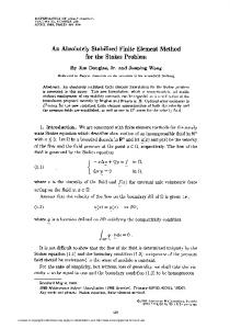
Plane strain Cook’s membrane problem
The Cook membrane problem is a bending dominated example that has been used by many authors as a reference test to check their element formulations. Here it will be used to compare results for the mixed and irreducible formulations in compressible elasticity, showing the behaviour of both bilinear quadrilateral and linear triangular elements. The problem consists of a tapered panel, clamped on one side and subjected to a shearing vertical load at the free end. Geometry of this plane strain problem is shown in Figure 1 (dimensions are in mm). For the evaluation of the stabilization parameters in the mixed formulation, L0 = 50 mm is taken as representative length of the problem. In order to test the convergence behaviour of the different formulations, the problem has been discretized into structured meshes with N finite elements along each side. Figures 2 and 3 compare the results obtained with four different spatial discretizations.
24
Figure 1: Geometry for the Cook membrane problem (dimensions are in mm) Figure 2 shows the relative convergence of the four discretizations on the computed value of the vertical displacement at the right top corner of the membrane (point A in Figure 1). Results are clearly different for the irreducible and the mixed elements and it is evident that the mixed formulation performs better for coarse and fine meshes. It also shows a slighter faster convergence rate. Figure 3 shows similar results on the computed value of the major principal stress at the mid-side point of the bottom boundary of the membrane (point B in Figure 1). It has to be noted that in order to compare stress values computed at the same point, the values reported for the irreducible elements correspond to the continuous projection Ph (C : ∇s uh ) evaluated at the mesh nodes, rather than the actual discontinuous stresses C : ∇s uh evaluated at the integration points. As it is well known, this projection procedure yields improved stress values for the irreducible formulation. Relative convergence characteristics on the stress values among the different elements compared are very similar to those observed for the displacements, and faster for the mixed formulation than for the irreducible one.
25
2.2
Q1/Q1 P1/P1 Q1 P1 best value
Vertical displacement at point A ( x E-10 )
2
1.8
1.6
1.4
1.2
1
0.8
0
10
20
30
40
50
60
70
Number of elements per side
Figure 2: Cook’s membrane problem. Vertical displacement at of point A versus number of elements along each side
4.5
Q1/Q1 P1/P1 Q1 P1 best value
4
Principal stress at point B
3.5
3
2.5
2
1.5
1
0
10
20
30
40
50
60
70
Number of elements per side
Figure 3: Cook’s membrane problem. Principal stress at point B versus number of elements along each side 26
5.2
Plane strain clamped arch problem
As a further illustration of the performance of the stabilized mixed ε/u formulation, we consider a clamped arch, of radius R = 10 and thickness t = 1, vertically loaded at the top (see Figure 4, dimensions are in m). Because of symmetry, only one half of the structure needs to be considered. The problem has been discretized into structured meshes consisting of N finite elements along the radial direction and 10N elements in the circumferential direction. Length L0 = t is taken as representative of the problem, for the evaluation of the stabilization parameters in the mixed formulation. As in the previous example, Figures 5 and 6 compare the results obtained with four different spatial discretizations: Q1/Q1, P 1/P 1, Q1and P 1. Figure 5 shows the relative convergence of the four discretizations used on the computed value of the vertical displacement under the point load (point A in Figure 4). In this case, the mixed interpolations also show improved performance over their irreducible formulations in the displacement results. Figure 6 shows results on the computed value of the major principal stress at point B on the outer face of the arch (see Figure 4). Again, the values reported for the irreducible elements correspond to the continuous projection Ph (C : ∇s uh ) evaluated at the mesh nodes. Again, the mixed formulations show better accuracy that the irreducible ones.
Figure 4: Geometry for the Clamped Arch problem
27
1.8
Q1/Q1 P1/P1 Q1 P1 best value
Vertical displacement at point A
1.6
1.4
1.2
1
0.8
0.6
0
5
10
15
20
25
30
35
40
Number of elements through thickness
Figure 5: Clamped arch problem. Vertical displacement of point A versus number of elements along the thickness
8
Q1/Q1 P1/P1 Q1 P1 best value
Horizontal tensile stress at point B
7
6
5
4
3
2
1
0
5
10
15
20
25
30
35
40
Number of elements through thickness
Figure 6: Clamped arch problem. Tensile principal stress at point B versus number of elements along the thickness 28
6
Conclusions
This paper presents the formulation of stable mixed stress/displacement and strain/displacement finite elements using equal order interpolation for the solution of nonlinear problems is solid mechanics. The proposed stabilization is based on the sub-grid scale approach and it circumvents the strictness of the inf-sup condition. The final method, consisting of stabilizing the standard formulation for mixed elements with the projection of the displacement symmetric gradient, yields an accurate and robust scheme, suitable for engineering applications in 2D and 3D. The derived procedure is also very general, independent of the constitutive equation considered. Numerical examples show that results compare favorably with the corresponding irreducible formulations, showing improved accuracy in the evaluation of the stress field. This characteristic is of great importance when facing nonlinear problems.
Acknowledgments Financial support from the Spanish Ministry for Education and Science under the SEDUREC project (CSD2006-00060) is acknowledged.
References [1] Fraeijs de Veubeke, B.X. Displacement and equilibrium models in the finite element method, in Stress Analysis, O.C. Zienkiewicz and G. Hollister, eds., Wiley (1965). [2] Malkus, D.S. and Hughes, T.J.R. Mixed finite element methods - reduced and selective integration techniques: a unification of concepts, Comp. Meth. in Appl. Mech. and Eng. (1978) 15, 63-81. [3] Arnold, D.N., Brezzi, F. and Fortin, M. A stable finite element for the Stokes equations. Calcolo (1984) 21, 337-344. [4] Simo, J.C., Taylor, R.L. and Pister, K.S. Variational and projection methods for the volume constraint in finite deformation elasto-plasticity, Comp. Meth. in Appl. Mech. and Eng. (1985) 51, 177-208.
29
[5] Simo, J.C. and Rifai, M.S. A class of mixed assumed strain methods and the method of incompatible modes, Int. Jour. for Num. Meths. in Eng. (1990) 29, 1595-1638. [6] Reddy, B.D. and Simo, J.C. Stability and convergence of a class of enhanced assumed strain methods, SIAM J. Num. Anal. (1995) 32, 17051728. [7] Bonet, J. and Burton, A.J. A simple average nodal pressure tetrahedral element for incompressible and nearly incompressible dynamic explicit applications. Comm. Num. Meths. in Eng. (1998)1 4, 437-449. [8] Zienkiewicz, O.C., Rojek, J., Taylor, R.L. and Pastor, M. Triangles and tetrahedra in explicit dynamic codes for solids, Int. J. for Num. Meths. in Eng. (1998) 43, 565-583. [9] Taylor, R.L. A mixed-enhanced formulation for tetrahedral elements, Int. Jour. for Num. Meths. in Eng. (2000) 47, 205-227. [10] Dohrmann, C.R., Heinstein, M.W., Jung, J., Key, S.W. and Witkowsky, W.R. Node-based uniform strain elements for three-node triangular and four-node tetrahedral meshes. Int. Jour. for Num. Meths. in Eng. (2000) 47, 1549-1568. [11] Bonet, J., Marriot, H. and Hassan, O. An averaged nodal deformation gradient linear tetrahedral element for large strain explicit dynamic applications. Comm. Num. Meths. in Eng. (2001) 17, 551-561. [12] Bonet, J., Marriot, H. and Hassan, O. Stability and comparison of different linear tetrahedral formulations for nearly incompressible explicit dynamic applications. Int. Jour. for Num. Meths. in Eng. (2001) 50, 119-133. [13] Oñate, E., Rojek, J., Taylor, R.L. and Zienkiewicz, O.C. Linear triangles and tetrahedra for incompressible problem usung a finite calculus formulation, Proceedings of European Conference on Computational Mechanics, ECCM, 2001. [14] de Souza Neto, E.A., Pires, F.M.A. and Owen D.R.J. A new F-barmethod for linear triangles and tetrahedra in the finite strain analysis 30
of nearly incompressible solids, Proceedings of VII International Conference on Computational Plasticity, COMPLAS, 2003. [15] Zienkiewicz, O.C. Taylor, R.L. Baynham, J.AW. Mixed and irreducible formulations in finite element analysis, in Hybrid and Mixed Finite Element Methods, S.N. Atlury, R.H. Gallagher and O.C. Zienkiewicz, eds.,Wiley (1983). [16] Zienkiewicz, O.C. and Taylor, R.L.. The Finite Element Method, Butterworth-Heinemann, Oxford, 2000. [17] Bischoff, M. and Bletzinger, K.-U. Improving stability and accuracy of Reissner-Mindlin plate finite elements via algebraic subgrid scale stabilizatio,. Comp. Meth. in Appl. Mech. and Eng. (2004) 193, 1517-1528. [18] Arnold, D.N. Mixed finite element methods for elliptic problems. Comput. Meth. Appl. Mech. Eng.(1990) 82, 281—300. [19] Brezzi, F. and Fortin, M. Mixed and Hybrid Finite Element Methods, Spinger, New York, 1991. [20] Brezzi, F., Fortin, M. and Marini, D. Mixed finite element methods with continuous stresses, Math. Models Meth. Appl. Sci. (1993) 3 ,275-287. [21] Mijuca, D. On hexahedral finite element HC8/27 in elasticity, Computational Mechanics (2004) 33, 466-480. [22] D.N. Arnold and R. Winther. Mixed finite elements for elasticity, Numerische Mathematik (2002) 92, 401-419. [23] D.N. Arnold, G. Awanou, and R. Winther. Finite elements for symmetric tensors in three dimensions, Math. Comput. (2008) 77, 1229-1251. [24] Hughes, T.J.R. Multiscale phenomena: Green’s function, Dirichlet-to Neumann formulation, subgrid scale models, bubbles and the origins of stabilized formulations, Comp. Meth. in Appl. Mech. and Eng. (1995) 127, 387-401. [25] Hughes, T.J.R., Feijoó, G.R., Mazzei. L., Quincy, J.B. The variational multiscale method-a paradigm for computational mechanics, Comp. Meth. in Appl. Mech. and Eng. (1998) 166, 3-28. 31
[26] Codina, R. and Blasco, J. A finite element method for the Stokes problem allowing equal velocity-pressure interpolations, Comp. Meth. in Appl. Mech. and Eng. (1997) 143, 373-391. [27] Codina, R. Stabilization of incompressibility and convection through orthogonal sub-scales in finite element methods, Comp. Meth. in Appl. Mech. and Eng. (2000) 190, 1579-1599. [28] Codina, R. Analysis of a stabilized finite element approximation of the Oseen equations using orthogonal subscales, Applied Numerical Mathematics (2008) 58, 264-283. [29] Codina, R. Finite element approximation of the three field formulation of the Stokes problem using arbitrary interpolations, SIAM Journal on Numerical Analysis (2009) 47, 699-718. [30] Badia, S. and Codina, R. Unified stabilized finite element formulations for the Stokes and the Darcy problems, SIAM Journal on Numerical Analysis, to appear. [31] Chiumenti, M., Valverde, Q., Agelet de Saracibar, C. and Cervera, M. A stabilized formulation for incompressible elasticity using linear displacement and pressure interpolations, Comp. Meth. in Appl. Mech. and Eng. (2002) 191, 5253-5264. [32] Cervera, M., Chiumenti, M., Valverde, Q. and Agelet de Saracibar, C. Mixed Linear/linear Simplicial Elements for Incompressible Elasticity and Plasticity, Comp. Meth. in Appl. Mech. and Eng. (2003), 192, 52495263. [33] Chiumenti, M., Valverde, Q., Agelet de Saracibar, C. and Cervera, M. A stabilized formulation for incompressible plasticity using linear triangles and tetrahedra, Int. J. of Plasticity (2004), 20 1487-1504. [34] Cervera, M., Chiumenti, M. and Agelet de Saracibar, C. Softening, localization and stabilization: capture of discontinuous solutions in J2 plasticity, Int. J. for Num. and Anal. Meth. in Geomechanics (2004), 28, 373-393.
32
[35] Cervera, M., Chiumenti, M. and Agelet de Saracibar, C. Shear band localization via local J2 continuum damage mechanic,. Comp. Meth. in Appl. Mech. and Eng. (2004), 193, 849-880. [36] Cervera, M. and Chiumenti, M. Size effect and localization in J2 plasticit, Comp. Meth. in Appl. Mech. and Eng. (2008), submitted. [37] Pastor, M., Li, T., Liu, X. and Zienkiewicz, O.C. Stabilized low-order finite elements for failure and localization problems in undrained soils and foundations, Comp. Meth. in Appl. Mech. and Eng. (1999), 174, 219-234. [38] Mabssout, M., Herreros, M.I. and Pastor, M. Wave propagation and localization problems in saturated viscoplastic geomaterials, Comp. Meth. in Appl. Mech. and Eng. (2003), 192, 955-971. [39] Mabssout, M. and Pastor, M. A Taylor-Galerkin algorithm for shock wave propagation and strain localization failure of viscoplastic continua, Int. Jour. for Num. Meths. in Eng. (2006) 68, 425-447. [40] Codina, R., Principe, J. and Baiges, J. Subscales on the element boundaries in the variational two-scale finite element method, Computer Methods in Applied Mechanics and Engineering (2009) 198, 838-852. [41] Badia, S. and Codina, R. Stabilized continuous and discontinuous Galerkin techniques for Darcy flow, submitted. E-prints UPC: http://upcommons.upc.edu/e-prints/handle/2117/2447. [42] Codina, R. Stabilized finite element approximation of transient incompressible flows using orthogonal subscales, Comp. Meth. in Appl. Mech. and Eng. (2002) 191, 4295-4321. [43] Baiocchi, C., Brezzi, F. and Franca, L. Virtual bubbles and Galerkin/least-squares type methods (Ga.L.S.), Comp. Meth. in Appl. Mech. and Eng. (1993) 105, 125-141. [44] Brezzi, F., Bristeau, M.O., Franca, L., Mallet, M. and Rogé, G. A relationship between stabilized finite element methods and the Galerkin method with bubble functions, Comp. Meth. in Appl. Mech. and Eng. (1992) 96, 117-129. 33
[45] Hughes, T.J.R., Franca, L.P. and Balestra, M. A finite element formulation for computational fluid dynamics: V. Circumventing the BabuskaBrezzi condition: A stable Petrov-Galerkin formulation of the Stokes problem accomodating equal-order interpolation, Comp. Meth. in Appl. Mech. and Eng. (1986) 59, 85-99. [46] Hughes, T.J.R., Franca, L.P. and Hulbert, G.M. A new finite element formulation for computational fluid dynamics: VIII. The Galerkin/leastsquare method for advective-diffusive equations, Comp. Meth. in Appl. Mech. and Eng. (1989) 73, 173-189. [47] Cervera, M., Agelet de Saracibar, C. and Chiumenti, M. COMET: COupled MEchanical and Thermal analysis. Data Input Manual, Version 5.0, Technical report IT-308, htpp://www.cimne.upc.es, 2002. [48] GiD: The personal pre and post preprocessor. htpp://www.gid.cimne.upc.es, 2002.
34