CYBERNETICS AND PHYSICS, VOL. 2, NO. 1, 2013 , 31–36
MIXED TRACKING AND PROJECTIVE SYNCHRONIZATION OF 5D HYPERCHAOTIC SYSTEM USING ACTIVE CONTROL
Kayode Ojo
Samuel Ogunjo
Oluwafemi Williams
Department of Physics University of Lagos, Akoka Nigeria
[email protected]
Condensed Matter and Statistical Physics Group Department of Physics Federal University of Technology Akure, Nigeria
[email protected]
Dept. of Physics FUT, Akure Nigeria
Abstract This paper examines mixed tracking control and hybrid synchronization of two identical 5-D hyperchaotic Lorenz systems via active control technique. The designed control functions for the mixed tracking enable each of the system state variables to stabilize at different chosen positions as well as control each state variables of the system to track different desired smooth function of time. Also, the active control technique is used to design control functions which achieve projective synchronization between the slave state variables and the master state variables. We also show that the coupling strength is inversely proportional to the synchronization time. Numerical simulations are carried out to validate the effectiveness of the analytical technique. Key words Hyperchaos, synchronization, tracking, active control. 1 Introduction Since the discovery of the first chaotic system by Lorentz in 1963 many new chaotic systems have been successively developed [Chen and Ueta, 1999; Chua and Lin, 1990; Qi et al, 2005; R¨ossler, 1976]. Chaos has gradually moved from simply being a scientific curiosity to a promising subject with practical significance and applications in different fields such as communication[Mengue and Essimbi, 2012], biological systems[Shi, 2012], economics and other fields. During the beginning of the last decade, one of the most fascinating discoveries that transformed research in the field of nonlinear dynamics and chaos theory is the fact that two or more chaotic systems evolving from different initial conditions can be made to synchronize, either by coupling the systems (locally or globally) or by forcing them. Synchronization means that the state
of a response system eventually approaches that of a driving system. This was first demonstrated by Pecora and Carroll [Pecora and Carroll, 1990]. Unrelenting research in chaotic systems has given rise to different types of synchronization including complete synchronization (CS) [Pecora and Carroll, 1990], generalized synchronization (GS) [Kacarev and Parlitz, 1996], projective synchronization (PS) [Mainieri and Rehacek, 1999], function projective synchronization (FPS)[An and Chen, 2008] amongst others. Chaotic behaviours could be beneficial feature in some cases, but can be undesirable in some engineering, biological and other physical applications; and therefore it is often desired that chaos should be controlled, so as to improve the system performance. Thus, it is of considerable interest and potential utility, to devise control techniques capable of forcing a system to maintain a desired dynamical behaviour even when intrinsically chaotic. The control of chaos and bifurcation is concerned with using some designed control input(s) to modify the characteristics of a parameterized nonlinear system. There might be need for different components of a chaotic system will be required to follow different trajectories when controlled, therefore, the need for mixed tracking or control. A number of methods such as OGY closed-loop feedback method [Ott, Grebogi and Yorke, 1990], active control [Bai and Lonngren, 1997], active backstepping [ Zhang, Ma, Li, and Zou, 2005] and recursive active control [Vincent, Laoye, and Odunaike, 2009] exist for the control of chaos in systems. Chaos control is considered as a special case of chaos synchronization. Despite the numerous advantages of mixed tracking, no research work has been done in this regard to the best of our understanding. The active control method introduced by [Bai and Lonngren, 1997] is efficient technique for the synchronization of chaotic systems because it can be used to
CYBERNETICS AND PHYSICS, VOL. 2, NO. 1, 2013
2 System Description The Lorenz system [Lorenz, 1963] was the first chaotic system to be modeled and one of the most widely studied. The original formula was modified into a 4D hyperchaotic system while Hu [Hu, 2009] constructed a 5-D hyperchaotic Lorenz system by introducing two state feedback to the classical 3-D Lorenz system. The new system, which can generate hyperchaotic attractors with three positive Lyapunov Exponents (LEs) is described by (1) x˙ 1 = −σx1 + σx2 + x4 x˙ 2 = rx1 − x2 + x1 x3 − x5 x˙ 3 = −βx3 + x1 x2 x˙ 4 = −x1 x3 + k1d x4
(1)
where σ, β, r are the parameters of the system and k1d , k2d are the bifurcation parameters. When parameters are set by default as σ = 10, β = 83 , r = 28, k1d = 2, k2d ϵ(2, 12), the system (1) behaves hyperchaotically with three positive LEs. The hyperchaotic attractor of the system is shown in figure (1). 3 Tracking Control of 5D Hyperchaotic Systems 3.1 Design of controllers We aim to design controllers that will enable (1) to be controlled to a predefined rule. To make it more flexible and adaptable, we preset the controls on each component of the 5D hyperchaotic system to different functions. The system (1) with the control parameters added are given as
y4
0
0 50 0 y2 −50 −50
50
−500 50 y3
y1
50
0
0
y5
500
−500 50
50 y3
Figure 1.
0 −50
50
0 0 −50
0 y2
−50 50
0 y5
0 y3 −50 0
50 y1
Attractors of 5-D hyperchaotic Lorenz system.
The error function is defined as e1 = x 1 − f 1 e2 = x 2 − f 2 e3 = x 3 − f 3 e4 = x 4 − f 4 e5 = x 5 − f 5
(3)
where fi are functions to be determined. Differentiating equation (3), we have e˙ 1 = x˙ 1 − f˙1 e˙ 2 = x˙ 2 − f˙2 (4)
e˙ 5 = x˙ 5 − f˙5 substituting (3) and (4) into (1), we have e˙ 1 = −σ(e1 + f1 ) + σ(e2 + f2 ) + (e4 + f4 ) + u1 − f˙1 e˙ 2 = r(e1 + f1 ) − (e2 + f2 ) − x1 x3 − (e5 + f5 ) + u2 − f˙2 e˙ 3 = −β(e3 + f3 ) + x1 x2 + u3 − f˙3 e˙ 4 = −x1 x3 + k1d (e4 + f4 ) + u4 − f˙4 e˙ 5 = k2d (e2 + f2 ) + u5 − f˙5 (5) eliminating terms which cannot be expressed as linear terms in e1 , e2 , e3 , e4 , e5 and solving for u(t), u1 = σf1 − σf2 − f4 + f˙1 + v1 (t) u2 = −rf1 + f2 + x1 x3 + f5 + f˙2 + v2 t
x˙ 1 = −σx1 + σx2 + x4 + u1 x˙ 2 = rx1 − x2 + x1 x3 − x5 + u2
x˙ 5 = k2d x2 + u5
500
e˙ 3 = x˙ 3 − f˙3 e˙ 4 = x˙ 4 − f˙4
x˙ 5 = k2d x2
x˙ 3 = −βx3 + x1 x2 + u3 x˙ 4 = −x1 x3 + k1d x4 + u4
50 y3
synchronize non-identical systems. The active control scheme has received considerable attention during the last decade. Applications to various systems abound some of which include Rossler and Chen system the electronic circuits which model a third-order ”jerk” equation Lorenz, Chen and Lu system geophysical model nuclear magnetic resonance (NMR) modeled by the nonlinear Bloch equations, RCL-shunted Josephson junction, inertial ratchets and most recently in extended Bonhoffer-Van der Pol oscillator. A chaotic system has been defined as one with sensitive dependence on initial condition and possess at least one positive Lyapunov exponent. An hyperchaotic system is one with more than one positive Lyapunov exponent[Li, 2012]. Notable hyperchaotic systems include [Kapitaniak and Chua, 1994; Ning and Haken, 1990; R¨ossler, 1979]
y4
32
(2)
u3 = βf3 − x1 x2 + f˙3 + v3 (t) u4 = x1 x3 − k1d f4 + f˙4 + v4 (t) u5 = −k2d f2 + f˙5 + v5 (t)
(6)
CYBERNETICS AND PHYSICS, VOL. 2, NO. 1, 2013 the parameter vi will be obtained later. Substituting (6) into (5), the differential of the error becomes
33
20 0 bsin(t)
−20
200 100
at2
0
e˙ 1 = −σe1 + σe2 + e4 + v1 (t) e˙ 2 = re1 − e2 − e5 + v2 (t) e˙ 3 = −βe3 + v3 (t)
40 3
constant
20
(7)
e˙ 4 = k1d e4 + v4 (t) e˙ 5 = k2d e2 + v5 (t)
100 0 −100 −200
c + dsin(t)
20 10 0 −10
2
at 0
Using the active control method, a constant matrix A is chosen which will control the error dynamics (7) such that the feedback matrix is e1 v1 (t) e2 v2 (t) v3 (t) = A e3 e4 v4 (t) v5 (t) e5
Figure 2.
5
10
15
20
25 Time
30
35
40
45
Components of 5D hyperchaotic Lorenz system when
controlled to different with different functions when the controls are
t = 20. The control functions are (a) tracking of f1 = b sin(t) by x1 , (b) tracking of f2 = at2 by x2 ,(c) tracking of f3 = k by x3 , (d) tracking of f4 = c + d sin(t) by x4 and (e) tracking of f5 = at2 by x5 . applied at time
(8)
Thus, the matrix A is chosen to be of the form
(λ1 + σ) −σ 0 −1 0 −r (λ2 + 1) 0 0 1 0 0 (λ + β) 0 0 A= 3 0 0 0 (λ4 + k1d ) 0 0 −k2d 0 0 λ5 (9) The eigenvalues λ1 , λ2 , λ3 , λ4 , λ5 are chosen to be negative.
4 Projective Synchronization of 5D System We define the master system as equation (1) and the slave system as y˙ 1 = −σy1 + σy2 + y4 + u1 (t) y˙ 2 = ry1 − y2 + y1 y3 − y3 + u2 (t) y˙ 3 = −βy3 + y1 y2 + u3 (t) y˙ 4 = −y1 y3 + k1d y4 + u4 (t) y˙ 5 = k2d y2 + u5 (t)
(10)
The goal of this synchronization is to determine the control function (u1 (t), u2 (t), u3 (t), u4 (t), u5 (t)). The error dynamics of the projective synchronization between (1) and (10) is defined as ei = yi − αxi
3.2
50
(11)
Numerical simulation
In the simulation, the fourth-order Runge-Kutta integration method is used to solve the differential equation with time step size equal to 0.0001 and the following initial conditions (x1 , x2 , x3 , x4 , x5 ) = (0, 1, 0, 1, 0). The system parameters are chosen as σ = 10, β = 8 3 , r = 28, k1d = 2, k2d ϵ(2, 12), so the system behaves hyperchaotically. We set f1 = b sin(t), f2 = at2 ,f3 = k, f4 = c + d sin(t) and f5 = at2 . Where b = 5, a = 0.1, c = 2, d = 50. The results are presented in figure (2). The effectiveness of the control can be seen as various components of the system converges to the preset functions when the controls are applied at time t > 0. Before the activation of the controls, the system behaves chaotically while the trajectory was changed to the present function on the activation of the control.
where i = 1, 2, . . . , 5 and α is the scaling factor. 4.1 Design of Control Functions By subtracting (1) from (10) and using the notation in (11), we obtain e˙ 1 = −σe1 + σe2 + e4 + u1 (t) e˙ 2 = re1 − e2 − e3 − y1 y3 + αx1 x3 + u2 (t) e˙ 3 = −βe3 + y1 y2 − αx1 x2 + u3 (t) e˙ 4 = k1d e4 − y1 y3 + αx1 x3 + u4 (t) e˙ 5 = k2d e2 + u5 (t)
(12)
To achieve asymptotic stability of system (12), we eliminate terms which cannot be expressed as linear
34
CYBERNETICS AND PHYSICS, VOL. 2, NO. 1, 2013
e1 e2 e3
u3 (t) = αx1 x2 − y1 y2 + v3 (t) u4 (t) = −αx1 x3 + y1 y3 + v4 (t)
100 0 −100 100 0 −100
e4
u1 (t) = v1 (t) u2 (t) = −αx1 x3 + y1 y3 + v2 (t)
100 0 −100
500 0 −500
e5
terms in e1 , e2 , e3 , e4 , e5 as follows:
200 0 −200
(13)
u5 (t) = v5 (t) substituting (13) into (12) e˙ 1 = −σe1 + σe2 + e4 + v1 (t) e˙ 2 = re1 − e2 − e3 + v2 (t) e˙ 3 = −βe3 + v3 (t) e˙ 4 = k1d e4 + v4 (t)
10
20
30
40
50
60
70
80
0
10
20
30
40
50
60
70
80
0
10
20
30
40
50
60
70
80
0
10
20
30
40
50
60
70
80
0
10
20
30
40 Time
50
60
70
80
(14) Figure 3. Error dynamics of the state variables when the control functions are activated for t ≥ 20.
e˙ 5 = k2d e2 + v5 (t) Using the active control method, a constant matrix A is chosen which will control the error dynamics (12) such that the feedback matrix is
60
40
20
(15)
with
x1, y1
v1 (t) e1 v2 (t) e2 v3 (t) = A e3 v4 (t) e4 v5 (t) e5
0
0
−20
−40
(λ1 + σ) −σ 0 −1 0 −σ (λ2 + 1) 0 0 1 0 0 (λ3 + β) 0 0 A= 0 0 0 (λ4 − k1d ) 0 0 −k2d 0 0 λ5 (16) In (16) the five eigenvalues λ1 , λ2 , λ3 , λ4 , λ5 are chosen to be negative in order to achieve a stable projective synchronization between two identical 5D hyperchaotic system. 4.2 Numerical simulation Numerical solutions were carried out using fourth order Runge-Kutta integration scheme to solve systems (1) and (10) with the following initial conditions (x1 , x2 , x3 , x4 , x5 ) = (0, 1, 0, 1, 0) and (y1 , y2 , y3 , y4 , y5 ) = (2, 2, 2, 2, 2). The system parameters are chosen as σ = 10, β = 83 , r = 28, k1d = 2, k2d ϵ(2, 12), so the system behaves hyperchaotically. The error dynamics of the system when the controls are activated at time t > 20 is shown in 3. The the synchronization errors between the two system is seen to converge to zero. Figures 4 - 8 shows the dynamics of the state variables (x and y) of the system when compared after activation of control at time t > 0 and value of α = 2.0. The trajectory of the master is seen to be twice that of the slave as expected. A quantity called
−60
0
10
20
30
40 Time
50
60
70
80
Figure 4. Dynamics of the state variable x1 and y1 when controls are activated at α = 2.0 and t ≥ 0.
synchronization time which gives a value of when the error between the two synchronization approaches zero was also computed. Figure (9) depicts the time it takes for synchronization to occur as the coupling strength is increased. From the graph, an exponential decrease is seen. This synchronization time-coupling strength graph can be used as a measure of the speed of synchronization. In effect, for the system under consideration the synchronization time is seen to decrease with increasing coupling strength. 5 Conclusion We have designed controllers for the control of 5Dhyperchaotic systems using active control and synchronization of identical 5D hyperchaotic Lorenz systems. From the results obtained, the tracking control was efficient and give practical results as each component of the system were designed to track different functions. Also, from the error dynamics, synchronization using
CYBERNETICS AND PHYSICS, VOL. 2, NO. 1, 2013
100
40
80
20
60 x3, y3
60
2 2
x ,y
35
0
40
−20
20
−40
0
−60
0
10
20
30
40 Time
50
60
70
80
Figure 5. Dynamics of the state variable x2 and y2 when controls are activated at α = 2.0 and t ≥ 0.
active control yield good results. Furthermore, the effectiveness of the control obtained was tested using the synchronization time - coupling strength graph. As the coupling strength increases, the synchronization time reduces. The synchronization times obtained are considered good for practical purposes. References An, H., and Chen, Y. (2008) The function cascade synchronization method and applications. Commun. Nonlinear Sci. Numer. Simul. 13, pp. 2246-2255. Bai E.W., and Lonngren K.E. (1997) Synchronization of two Lorenz systems using active control, Chaos, Solitons & Fractals, 8, pp. 51–58. Chen, G., and Ueta, T. (1999) Yet another chaotic attractor, Int. Journal of Bifurcation and Chaos, 9(7), pp. 1465-1466. Chua, L.O., and Lin, G.N (1990) Canonical realization of Chua’s circuit family, IEEE Transactions on Circuits and Systems, 37(7), pp. 885-902. Hu., G. (2009) Generating hyperchaotic attractors with three positive Lyapunov exponents via state feedback control. Int. Journal of Bifurcation and Chaos.
−20
0
10
20
30
40 Time
50
60
70
80
Figure 6. Dynamics of the state variable x3 and y3 when controls are activated at α = 2.0 and t ≥ 0.
Hongwei, Li (2012) Dynamical analysis in a 4D hyperchaotic system, Nonlinear Dyn. 70, pp. 1327-1334. Kacarev, L., and Parlitz, U. (1996) Generalized synchronization, predictability, and equivalence of unidirectionally coupled dynamical systems. Phys. Rev. Lett. 76, pp. 1816-1819. Kapitaniak, T., and Chua, L.O (1994) Hyperchaotic attractor of unidirectionally coupled Chua’s circuit. Int. J. Bifurc. Chaos Appl. Sci. Eng. 4, pp. 477-482. Lorenz (1963) Deterministic nonperiodic flow. J. Atmos. Phys. 20, pp. 131–141. Mainieri, R., and Rehacek, J. (1999) Projective synchronization in the three-dimensional chaotic systems. Phys. Rev. Lett. 82, pp. 3042-3045. Mengue, A.D., and Essimbi, B.Z (2012) Secure communication using chaotic synchronization in mutually coupled semiconductor lasers, Nonlinear Dyn. 70, pp. 1241-1253. Ning, C., and Haken, H. (1990) Detuned lasers and the complex Lorenz equations: Subcritical and supercritical Hopf bifurcations. Phys. Rev. A 41, pp. 38263837. Ott, E. Grebogi,C. and Yorke J. A. (1990) ”Controlling
36
CYBERNETICS AND PHYSICS, VOL. 2, NO. 1, 2013
400 300
150
200 100
0
50
4
x ,y
4
100
x5, y5
−100 −200 −300
0
−50
−400 −500
−100 0
10
20
30
40 Time
50
60
70
80 −150
Chaos,” Phys. Rev. Lett. 64 (1990) 1196–1199. Pecora, L.M., and Carroll, T.L. (1990) Synchronization in chaotic systems, Phys. Rev. Lett. 64, pp. 821–824. Qi, G., Chen, G., Du, S., Chen, Z., and Yuan, Z. (2005) Analysis of a new chaotic system, Physica A, 352(24), pp. 295-308. R¨ossler, O.E. (1976) An equation for continuous chaos, Physics Letters A, 57(5), pp. 397-398. R¨ossler, O.E. (1979) An equation for hyperchaos. Phys. Lett. A, 71, pp. 155-157. Yanxiang, Shi (2012) Chaos and Control in Coronary Artery System, Discrete Dynamics in Nature and Society, Article ID 631476. Vincent, U.E., Laoye, J.A., and Odunaike, R.K. (2009) Chaos control in the nnonlinear Bloch equations using recursive active control. African Journal Of Mathematical Physics, 7(1), pp. 31–38. Zhang, H., Ma, X.-K., Li, M., and Zou, J.-L. (2005) Control and tracking hyperchaotic R¨ossler system via active backstepping design, Chaos, Solitons & Fractals, 26, pp. 353–361.
10
20
30
40 Time
50
60
70
80
Figure 8. Dynamics of the state variable x5 and y5 when controls are activated at α = 2.0 and t ≥ 0.
10 9 8 Synchronization time
Figure 7. Dynamics of the state variable x4 and y4 when controls are activated at α = 2.0 and t ≥ 0.
0
7 6 5 4 3 2 1 0
0
Figure 9.
5
10 λ
15
20
Dependence of the synchronization time on the coupling
parameter λ.