Mixtures of Deterministic-Probabilistic Networks and their AND

120

DECHTER & MATEESCU

UAI 2004

Mixtures of Deterministic-Probabilistic Networks and their AND/OR Search Space

Rina Dechter and Robert Mateescu School of Information and Computer Science University of California, Irvine, CA 92697-3425 {dechter, mateescu}@ics.uci.edu

Abstract The paper introduces mixed networks, a new framework for expressing and reasoning with probabilistic and deterministic information. The framework combines belief networks with constraint networks, defining the semantics and graphical representation. We also introduce the AND/OR search space for graphical models, and develop a new linear space search algorithm. This provides the basis for understanding the benefits of processing the constraint information separately, resulting in the pruning of the search space. When the constraint part is tractable or has a small number of solutions, using the mixed representation can be exponentially more effective than using pure belief networks which model constraints as conditional probability tables.

1 INTRODUCTION Modeling real-life decision problems requires the specification and reasoning with probabilistic and deterministic information. The primary approach developed in artificial intelligence for representing and reasoning with partial information under conditions of uncertainty is Bayesian networks. They allow expressing information such as “if a person has flu, he is likely to have fever.” Constraint networks and propositional theories are the most basic frameworks for representing and reasoning about deterministic information. Constraints often express resource conflicts frequently appearing in scheduling and planning applications, precedence relationships (e.g., “job 1 must follow job 2”) and definitional information (e.g., “a block is clear iff there is no other block on top of it”). Most often the feasibility of an action is expressed using a deterministic rule between the pre-conditions (constraints) and post-conditions that must hold before and after executing an action (e.g., STRIPS for classical planning).

The two communities of probabilistic networks and constraint networks matured in parallel with only minor interaction. Nevertheless some of the algorithms and reasoning principles that emerged within both frameworks, especially those that are graph-based, are quite related. Both frameworks can be viewed as graphical models, a popular paradigm for knowledge representation. Researchers within the logic-based and constraint communities have recognized for some time the need for augmenting deterministic languages with uncertainty information, leading to a variety of concepts and approaches such as non-monotonic reasoning, probabilistic constraint networks and fuzzy constraint networks. The belief networks community started only recently to look into mixed representation [Poole1993, Ngo & Haddawy1977, Dechter & Larkin2001] perhaps because it is possible, in principle, to capture constraint information within belief networks [Pearl1988]. Indeed, constraints can be embedded within belief networks by modeling each constraint as a Conditional Probability Table (CPT). One approach is to add a new variable for each constraint that is perceived as its effect (child node) in the corresponding causal relationship and then to clamp its value to true [Pearl1988]. While this approach is semantically coherent and complies with the acyclic graph restriction of belief networks, it adds a substantial number of new variables, thus cluttering the problem’s structure. An alternative approach is to designate one of the arguments of the constraint as a child node (namely, as its effect). This approach, although natural for functions (the arguments are the causes or parents and the function variable is the child node), is quite contrived for general relations (e.g., x+ 6 6= y). Such constraints may lead to cycles, which are disallowed in belief networks. Furthermore, if a variable is a child node of two different CPTs (one may be deterministic and one probabilistic) the belief network definition requires that they be combined into one CPT. The main shortcoming, however, of any of the above integrations is computational. Constraints have special properties that render them attractive computationally. When con-

UAI 2004

DECHTER & MATEESCU

straints are disguised as probabilistic relationships, their computational benefits are hard to exploit. In particular, the power of constraint inference and constraint propagation may not be brought to bear. Therefore, we propose a framework that combines deterministic and probabilistic networks, called mixed network. Specifically, we propose a mixed network framework in which the identity of the respective relationships, as constraints or probabilities, will be maintained explicitly, so that their respective computational power and semantic differences can be vivid and easy to exploit. The mixed network approach allows two distinct representations: causal relationships that are directional and normally (but not necessarily) quantified by CPTs and symmetrical deterministic constraints. The proposed scheme’s value is in providing: 1) semantic coherence; 2) user-interface convenience (the user can relate better to these two pieces of information if they are distinct); and most importantly, 3) computational efficiency.

2 PRELIMINARIES AND BACKGROUND Reasoning graphical model A reasoning graphical model is a triplet R = (X, D, F ) where X is a set of variables, X = {X1 , . . . , Xn }, D = {D1 , . . . , Dn } is the set of their respective finite domains and F = {F1 , . . . , Ft } is a set of real-valued functions, defined over subsets of X. The primal graph of a reasoning problem has a node for each variable, and any two variables appearing in the same function’s scope are connected. The scope of a function is its set of arguments. Belief networks A belief network can be viewed as an instance of a reasoning graphical model. In this case the set of functions F is denoted by P = {P1 , . . . , Pn } and represents a set of conditional probability tables (CPTs): Pi = P (Xi |pai ). pai are the parents of Xi . When the CPTs entries are “0” or “1” only, they are called deterministic or functional CPTs. The associated directed graph G, drawn by pointing arrows from parents to children, should be acyclic. We also denote belief networks by B = (X, D, G, P ). The belief network represents a probability distribution over X having the product form PB (¯ x) = P (x1 , . . . , xn ) = Πni=1 P (xi |xpai ) where an assignment x¯ = (X1 =x1 , . . . , Xn =xn ) is abbreviated to x ¯ = (x1 , . . . , xn ) and where xS or x[S] denote the restriction of a tuple x over a subset of variables S. An evidence set e is an instantiated subset of variables. We use upper case letters for variables and nodes in a graph and lower case letters for values in a variable’s domain. The moral graph of a directed graph is the undirected graph obtained by connecting the parent nodes of each variable and eliminating direction. Given a directed graph G, the ancestral graph relative to a subset of nodes X is the undirected graph obtained by taking the subgraph of G that contains X and all their non-descendants, and moralizing the graph.

121

Constraint networks A constraint network can also be viewed as an instance o a reasoning graphical model. In this case the functions are denoted by C = {C1 , ..., Ct }, and the constraint network is denoted by R = (X, D, C). Each constraint is a pair Ci = (Si , Ri ), where Si ⊆ X is the scope of the relation Ri defined over Si , denoting the allowed combinations of values. The associated graph G of a constraint network R is its primal graph. We say that R represents its set of solutions, ρ, or ρ(R). A particular example of constraint networks is CNF, in which the variables are boolean (binary domains) and the constraints are boolean formulas. In this case the network is given as formula in conjunctive normal form. Induced-graphs and induced width An ordered graph is a pair (G, d) where G is an undirected graph, and d = X1 , ..., Xn is an ordering of the nodes. The width of a node in an ordered graph is the number of the node’s neighbors that precede it in the ordering. The width of an ordering d, denoted w(d), is the maximum width over all nodes. The induced width of an ordered graph, w∗ (d), is the width of the induced ordered graph obtained as follows: nodes are processed from last to first; when node X is processed, all its preceding neighbors are connected. The induced width of a graph, w∗ , is the minimal induced width over all its orderings. The tree-width of a graph is the minimal induced width. Tasks The primary queries over belief networks are: belief updating, evaluating the posterior probability of each singleton proposition given some evidence; most probable explanation (MPE), finding a complete assignment to all variables having maximum probability given the evidence and maximum a posteriori hypothesis (MAP), which calls for finding the most likely assignment to a subset of hypothesis variables given the evidence. The primary queries over constraint networks are to decide if the network is consistent and if so, to find one, some or all solutions.

3 MIXING PROBABILITIES WITH CONSTRAINTS D EFINITION 1 (mixed networks) Given a belief network B = (X, D, G, P ) that expresses the joint probability PB and given a constraint network R = (X, D, C) that expresses a set of solutions ρ, a mixed network based on B and R denoted M(B,R) = (X, D, G, P, C) is created from the respective components of the constraint network and the belief network as follows. The variables X and their domains are shared, (we could allow non-common variables and take the union), and the relationships include the CPTs in P and the constraints in C. The mixed network may be inconsistent, or if it is consistent it expresses the conditional probability PM (X):  PB (¯ x|x ¯ ∈ ρ), if x ¯∈ρ PM (¯ x) = 0, otherwise.

122

DECHTER & MATEESCU

Belief updating, MPE and MAP queries can be extended to mixed networks straightforwardly. They are well defined relative to the mixed probability PM , when the constraint portion is consistent. An additional relevant query over a mixed network is to find the probability that a random tuple satisfies the constraint query, namely PB (¯ x ∈ ρ). The auxiliary network We now define the belief network that expresses constraints as pure CPTs. D EFINITION 2 (auxiliary network) Given a mixed network M(B,R) we define the auxiliary network S(B,R) to be a belief network that has new auxiliary variables as follows. For every constraint Ci = (Si , Ri ) in R, we add the auxiliary variable Ai that has a domain of two values, {0, 1}. There is a CPT defined over Ai whose parent variables are Si , defined as follows: P (Ai =1 | tSi ) =



1, 0,

if t ∈ Ri otherwise.

S(B,R) is a belief network that expresses a probability distribution PS . It is easy to see that, Proposition 1 Given a mixed network M(B,R) and an associated auxiliary network S = S(B,R) , then: PM (¯ x) = PS (¯ x|A1 =1, ..., At =1). One source of determinism in the context of belief networks may arise because we have deterministic queries or complex evidence description. Both reduce to CNF or Constraint Probability Evaluation (CPE). D EFINITION 3 (CPE) Given a mixed network M(B,R) , where the belief network (X, D, G, P ) is defined over variables X = {X1 , ..., Xn } and where the constraint portion is a either a set of relational constraints or a CNF query (R = ϕ) over a subset Q = {Q1 , ...Qr }, where Q ⊆ X, the Constraint, respectively CNF, Probability Evaluation (CPE) task is to find the probability PB (¯ x ∈ ρ(R)), respectively PB (¯ x ∈ m(ϕ)) where m(ϕ) are the models (solutions of ϕ) . Alternatively, we can envision situations when one wants to assess the belief of a proposition given partial, disjunctive information. Belief assessment conditioned on a CNF evidence is the task of assessing P (X|ϕ) for every variable X. Since P (X|ϕ) = αP (X ∧ ϕ) where α is a normalizing constant relative to X, computing P (X|ϕ) reduces to a CPE task for the query ((X = x) ∧ ϕ). More generally, P (ϕ|ψ) can be derived from P (ϕ|ψ) = αϕ · P (ϕ ∧ ψ) where αϕ is a normalization constant relative to all the models of ϕ.

UAI 2004

4 MIXED GRAPHS AS I-MAPS In this section we define the mixed graph of a mixed network and an accompanying separation criterion, extending d-separation. We show that a mixed graph is a minimal Imap (independency map) of a mixed network relative to an extended notion of separation, called dm-separation. D EFINITION 4 (A mixed graph) Given a mixed network M(B,R) , the mixed graph GM = (GB , GR ) is defined as follows. Its nodes are the set of variables X, and the arcs are the union of the directed arcs in the belief network graph GB and the undirected arcs in the constraint graph GR . The moral mixed graph is the union of the moral graph of the belief network, and the constraint graph. The notion of d-separation in belief networks is known to capture conditional independence [Pearl1988]. Namely any d-separation in the directed graph corresponds to a conditional independence in the corresponding probability distribution. Likewise, an undirected graph representation of probabilistic networks (e.g., Markov networks) allows reading valid conditional independence based on undirected graph separation. In this section we define dm-separation for mixed graphs and show that it provides a criterion for establishing minimal I-mapness for mixed networks. D EFINITION 5 (ancestral graphs in mixed networks) Given a mixed graph GM = (GB , GR ) of a mixed network M(B,R) where GB is the directed graph of B, and GR is the undirected constraint graph of R, the ancestral graph of Y ⊆ X in GM is the union of GR and the ancestral graph of Y in GB . D EFINITION 6 (dm-separation) Given a mixed graph, GM and given three subsets of variables W , Y and Z which are disjoint, we say that W and Y are dm-separated given Z in the mixed graph GM , denoted hW, Z, Y idm , iff in the ancestral mixed graph of W ∪ Y ∪ Z, all the paths between W and Y are intercepted by variables in Z. T HEOREM 1 (I-map) Given a mixed network M = M(B,R) and its mixed graph GM , then GM is a minimal I-map relative to dm-separation. Namely, if hW, Z, Y idm then PM (W |Y, Z) = PM (W |Z) and no arc can be removed while maintaining this property. Example 1 Figure 1(a) shows a regular belief network in which W and Y are d-separated given the empty set. If we add a constraint RP Q between P and Q, we obtain the mixed network in Figure 1(b). According to dm-separation W is no longer independent of Y given the empty set, because of the path W P QY in the ancestral graph. Figure 1(c) shows the auxiliary network, with variable A assigned

UAI 2004

DECHTER & MATEESCU

W

Y

W

Y

W

Y

P

Q

P

Q

P

Q

Z

Z

(a)

(b)

A

Z

(c)

Figure 1: dm-separation in mixed networks to 1 corresponding to the constraint between P and Q. Dseparation also dictates a dependency between W and Y , given A = 1. We will next see the first virtue of mixed vs auxiliary networks. It is now clear that the concept of constraint propagation has a well defined meaning within the mixed network framework. That is, we can allow the constraint network to be processed by any constraint propagation algorithm to yield another, equivalent, mixed network. D EFINITION 7 (equivalent mixed networks) Two mixed networks defined on the same set of variables X = {X1 , ..., Xn } and the same domains, D1 , ..., Dn , denoted M1 = M(B1 ,R1 ) and M2 = M(B2 ,R2 ) , are equivalent iff they are equivalent as probability distributions, namely iff PM1 = PM2 . Proposition 2 If R1 and R2 are equivalent constraint networks (have the same set of solutions), then M(B,R1 ) is equivalent to M(B,R2 ) . The above proposition shows one advantage of looking at mixed networks rather than at auxiliary networks. Due to the explicit representation of deterministic relationships, notions such as inference and constraint propagation are naturally defined and exploitable in mixed network.

5 AND/OR SEARCH SPACES FOR GRAPHICAL MODELS

123

In contrast to inference algorithms which exploit the independencies in the underlying graphical model effectively (e.g. variable elimination, tree-clustering), the OR search space does not capture any of the structural properties of the underlying graphical model. Introducing AN D nodes into the OR search space can capture the graph-model structure by decomposition the problem into independent subproblems. The AND/OR search space is a well known problem solving approach developed in the area of heuristic search, that exploits the problem structure to decompose the search space. The states of an AND/OR space are of two types: OR states which usually represent alternative ways of solving the problem, and AND states which usually represent problem decomposition into subproblems, all of which need to be solved. We will next present the AND/OR search space for a general reasoning graphical model which in particular applies to mixed networks. For more details see [Dechter2004]. For illustration consider the simple tree graphical model in Figure 2a, over domains {1, 2, 3} which represents a graphcoloring problem. Once variable X is assigned the value 1, the search space it roots corresponds to two independent subproblems, one that is rooted by Y and the other rooted by Z. These two search subspaces do not interact. This can be captured by viewing the assignment hX, 1i as an AND state, having two descendants. One is labeled by variable Y and the other by variable Z. The same decomposition can be associated with the other assignments to X. Applying the decomposition recursively to Y and Z and so on along the tree (Figure 2a) yields the AND/OR search tree in Figure 2c. Notice that in the AND/OR space a full assignment to all the variables is not a path in the search space but a subtree. A solution subtree is highlighted in 2c. Clearly, the size of the AND/OR search space can be far smaller than that of the regular OR space (compare the number of states in 2b with that in 2c). 5.1 AND/OR SEARCH TREES

One way of taking advantage of the implications of Proposition 2 is by search. The intuitive idea for mixed networks is to search in the space of partial variable assignments, and use the constraints to limit the actual searched space. This sections introduces the basics of a new AND/OR search space paradigm for graphical models. The usual way to do search (called here OR search) is to instantiate variables in turn (in a static or dynamic ordering). In the most simple case this defines a search tree, whose nodes represent states in the space of partial assignments, and the typical depth first (DFS) algorithm searching this space would require linear space. If more space is available, then some of the traversed nodes can be cached, and retrieved when encountered again, and the DFS algorithm would in this case traverse a graph rather than a tree.

The definition of an AND/OR space is not restricted to tree graph-models, however it has to be guided by a tree which spans the original graph-model. We can use a DFS spanning tree. Given a DFS traversal of a graph G, the corresponding DFS spanning tree T is defined by taking only the traversed arcs of G. Given a reasoning graphical model R, its primal graph G and a DFS tree T of G, the associated AND/OR tree is defined as follows. The AND/OR search tree has alternating levels of AND and OR nodes. The OR nodes are labeled Xi and correspond to the variables. The AND nodes are labeled hXi , vi and correspond to the values v assigned to Xi . The structure of the AND/OR search tree is based on the underlying DFS tree T . The root of the AND/OR search

124

DECHTER & MATEESCU

UAI 2004

X

OR X

3

2

1

AND Y

T

2

2

1

3

1

1

3

1

3

2

2

3

2

1

2

1

3

1

3

2

Z

Y

OR

3

Y

Z

Y

Z

X R

Z

Y

Z

2

1

3

1

3

2

3

2

3

1

2

1

2

1

2

1

2

2

3

2

3

AND

T

M

L

R

1

3

1

AND

3

M

L

2

1

3

1

3

1

1

2

(c) AND/OR search tree with one of its solution subtrees

(b) OR search tree

(a) A constraint tree

3

3

1

M

2

R

T

OR L

3

2

3

Figure 2: OR vs. AND/OR search trees; note the connector for AND arcs X

X Y

3

2

1

Z

Y

T R

1

Z

2

1

3

1

2

1

3

3

2

1

3

2

1

3

2

2

2

3

1

M

1

1

2

3

1

2

2

1

3

2

3

2

1

T

R

T

L

Z

Y

Z

Y

3

1

3

2

3

2

2

1

3

1

3

2

1

R

T

R

L

L

M

M

L

M

3

3

1

2

3

1

2

3

1

2

3

1

2

3

Figure 3: Condensed OR graph for the tree problem

Figure 4: AND/OR search graph for the tree problem

tree is an OR node, labeled with the root of T . The children of an OR node Xi are AND nodes labeled with its possible assignments hXi , vi. The children of an AND node hXi , vi are OR nodes labeled with the children of variable Xi in the DFS tree T . The value of leaf nodes is ”S” (solved) if they represent a partial consistent assignment, or ”U” if they corresponds to a dead-end.

depth of the underlying DFS tree T . Therefore, DFS trees of smaller height are better. However, there is a larger class of spanning trees that can be used to derive AND/OR search trees, called legal trees, which have the above mentioned back-arc property.

A solution subgraph of an AND/OR search graph G is a subtree which: (1) contains the start node s0 ; (2) if n in the subtree is an OR node then it contains one of its child nodes in G and if n is an AND node it contains all its children in G; (3) all its terminal nodes are ”Solved” (S). If we look at a probabilistic network that expresses a positive probability distribution each full assignment will be expressed as ”Solved” in the AND/OR search tree. When a depth-first search algorithm is applied to the AND/OR search tree, it requires linear space, storing only the current path from root. It is therefore important that during the search, the scope of every function from F be fully assigned on some path. The DFS tree T of G has the property that if we add to T all the other arcs of G which do not appear in T , only back-arcs (i.e. arcs between a node and one of its ancestor) will be created. In other words no arcs will be added between different branches of T , which ensures that each scope of F will be fully assigned on some path in T . The size of the AND/OR search tree will depend on the

D EFINITION 8 (legal tree of a graph) Given an undirected graph G = (V, E), a directed rooted tree T = (V, E 0 ) defined on all its nodes is legal if any arc of G which is not included in E 0 is a back-arc, namely it connects a node to an ancestor in T . The arcs in E 0 may not all be included in E. Given a legal tree T of G, the extended graph of G relative to T is defined as GT = (V, E ∪ E 0 ). Clearly, any DFS tree and any chain are legal trees. Searching the OR space corresponds to searching a chain-based space, which is a special legal tree. It is easy to see that the size of the AND/OR tree is exponential in the depth of the legal tree. Therefore, any algorithm searching this space is bounded by that complexity. Finding a legal or a DFS tree of minimal depth is known to be NP-complete. However the problem was studied, and various greedy heuristics are available. The following relationship between the induced-width and the depth of legal trees is well known [Bayardo & Miranker1996, Dechter2003]. Given a treedecomposition of a primal graph G having n nodes, whose tree-width is w∗ , there exists a legal tree T of G whose depth, m, satisfies: m ≤ w∗ · log n. In summary,

UAI 2004

DECHTER & MATEESCU

T HEOREM 2 ([Dechter2004]) Given a graphical model R and a legal tree T , its AND/OR search tree ST (R) is sound and complete (contains all and only solutions) and its size is O(n·exp(m)) where m is the legal tree’s depth. A graphical model that has a tree-width w∗ has an AND/OR search tree whose size is O(exp(w∗ · log n)). 5.2 AND/OR SEARCH GRAPHS It is often the case that certain states in the search tree can be merged because the subtree they root are identical. Any two such nodes are called unifiable, and when merged, transform the search tree into a search graph. 5.2.1 Minimal AND/OR Search Graphs A partial path in the AND/OR search-tree ST ¯ a (hX1 , a1 i, hX2 , a2 i, ..., hXi , ai i) is abbreviated to (X, ¯i ), ¯ where X is the sequence of variables and a ¯ is their corresponding sequence of value assignments. D EFINITION 9 (legal transformation) Given two partial ¯i, a paths over the same set of variables, s1 = (X ¯i ), s2 = ¯ ¯ (Xi , bi ) where ai = bi = v, we say that s1 and s2 are unifiable at hXi , vi (can be merged) iff the search subgraphs rooted at s1 and s2 are identical. The Merge operator over search graphs, M erge(s1 , s2 ) transforms ST into a graph ST0 by merging s1 with s2 . It can be shown that the closure under the merge operator of an AND/OR search space yields a unique fixed point, D EFINITION 10 (minimal AND/OR search graph) The minimal AND/OR search graph relative to T is the closure under merge of the AND/OR search tree ST . The above definition is applicable, via the legal-chain definition, to the traditional OR search tree as well, however, its compression is inferior, because of the linear structure imposed by the OR search tree. This distinction will be clarified shortly. Example 2 The smallest OR search graph of the search tree in Figure 2(b) is given in Figure 3. The smallest AND/OR graph of the same problem along some DFS tree is given in Figure 4. We see that some variable-value pairs must be repeated in Figure 3 while in an AND/OR case they appear just once. For example, the subgraph below the paths hX, 1i, hY, 2i and hX, 3i, hY, 2i in Figure 3 cannot be merged. 5.2.2 Rules for Merging Nodes Given a reasoning graphical model R = (X, D, F ) and a legal tree T , there could be many AND/OR graphs relative to T that are equivalent to the AND/OR search tree

125

ST , each obtained by some sequence of merging. The following rules provide an efficient way for generating such graphs without creating the whole search tree first. The rules are based on a definition of induced-width of a legal tree of G which is instrumental for characterizing OR graphs vs. AND/OR graphs. We denote by ddf s (T ) a DFS ordering of a tree T . D EFINITION 11 (generalized induced-width of a legal tree) Given GT , an extended graph of G relative to T (see definition 9), the generalized induced width of G relative to legal tree T , wT (G) is the induced-width of GT along ddf s (T ). We can show that, 1. The minimal generalized inducedwidth of G relative to all legal trees is identical to the induced-width (tree-width) of G. 2. The generalized induced-width of a legal chain d is identical to its pathwidth pw(d) along d. Given an induced graph of GT , denoted G∗ T along ddf s (T ), each variable and its parent set is a clique. D EFINITION 12 (parents, parent-separators) Given the induced-graph, G∗ T , the parents of X denoted psX , are its earlier neighbors in the induced-graph. Its parentseparators, psaX are its parents that are also neighbors of future variables relative to X, in T . Note that for every node except those latest in the cliques of the induced graph, the parent-separators are identical to the parents. For nodes latest in cliques, the parent-separators are the separators between cliques. In G∗ T , for every node Xi , the parent-separators of Xi separates in T its ancestors on the path from the root, and all its descendents in GT . The reader should compare Figures 3 and 4 to verify merging using context. T HEOREM 3 [Dechter2004] Given G∗ T , let s1 = (¯ ai , hXi+1 , vi) and s2 = (¯bi , hXi+1 , vi) be two partial paths of assignments in its AND/OR search tree ST , ending with the same assignment variable hXi+1 , vi. If projecting s1 and s2 on the parent separators psai+1 is identical, namely: s1 [psai+1 ] = s2 [psai+1 ], then the AND/OR search subtrees rooted at s1 and s2 are identical and s1 and s2 can be merged at hXi+1 , vi. D EFINITION 13 (context) For every state si , si [psai ] is called the context of si when psai is the parent-separators set of Xi relative to the legal tree T . T HEOREM 4 [Dechter2004] Given G, a legal tree T and its induced width w = wT (G), the size of the AND/OR search graph based on T obtained when every two nodes in ST having the same context are merged is O(n · k w ), when k bounds the domain size.

126

DECHTER & MATEESCU

AND-OR- CPE () Input: A mixed network M(B,R) = (X, D, G, P, C). A DFS tree T rooted at X1 of the moral mixed graph of M(B,R) . Output: The probability P (¯ x ∈ ρ(R)) that a tuple satisfies the constraint query. (1) Initialize OPEN by adding X1 to it (X1 is an OR node); PATH := φ (2) if OPEN == φ return g(X1 ) Remove the first node in OPEN, call it n Add n to PATH (3) Expand n generating all its successors as follows: if (n is an OR node, denote n by Xi ) g(Xi ) := 0 succ(Xi ) := {hXi , vi | relevant constraints Cj , s.t. scope(Cj ) ⊆ PATH ∪ {hXi , vi}, are satisfied } else (n is an AND node, denote n by hXi , vi) g(hXi , vi) := 1 A := {P (Y |paY ) | (Xi ∈ paY ∪ {Y }) and (paY ∪ {Y } ⊆ PATH)} (CPTs with fully assigned scope containing Xi ) if A 6= φ Q g(hXi , vi) := g(hXi , vi) ∗ A P (Y = y | paY ), if g(hXi , vi) == 0 succ(hXi , vi) := φ else succ(hXi , vi) := Children(Xi ) in T Add succ(n) on top of OPEN (4) while succ(n) == φ (a) if (n is an OR node) g(P arent(n)) := g(P arent(n)) ∗ g(n) if (g(n) == 0) remove succ(P arent(n)) from OPEN succ(P arent(n)) := φ (b) if (n is an AND node) g(P arent(n)) := g(P arent(n)) + g(n) succ(P arent(n)) := succ(P arent(n)) − {n} remove n from PATH n := Last(PATH) (5) go to step (2)

Figure 5: Algorithm AND-OR- CPE Thus, the minimal AND/OR search graph of G relative to T is O(n · k w ) where w = wT (G). Since minT {wT (G)} equals w∗ and since minT ∈chains {wT (G)} equals pw∗ , Corollary 1 The minimal AND/OR search graph is bounded exponentially by the primal graph’s tree-width while the OR minimal search graph is bounded exponentially by its path-width. It is known [Bodlaender & Gilbert1991] that for any graph w∗ ≤ pw∗ ≤ w∗ · log n. It is also easy to place m∗ (the minimal depth legal tree) yielding w∗ ≤ pw∗ ≤ m∗ ≤ w∗ · log n. The difference between tree-width and path-width can be substantial. In fact for balanced trees the tree-width is 1 while the path-width is log n, where n is the number of variables, yielding a substantial difference between OR and AND/OR search graphs.

A

UAI 2004

C

C

D

OR

A

B

B

D

AND OR

C

AND OR

ϕ = ( A ∨ ¬B)( D ∨ ¬C )

(a)

AND 0

(b)

A 0

1

1

0

1

B

D

B

D

1

0

0

(c)

Figure 6: a) Mixed network; b) DFS tree; c)AND/OR search tree

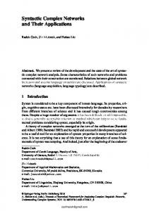
6 ALGORITHMS FOR PROCESSING MIXED NETWORKS We will focus on the CPE task of computing P (¯ x ∈ ρ(R)), the probability that a random tuple satisfies the constraint query. A number of related tasks can be easily derived by changing the appropriate operator (e.g., using maximization for maximum probable explanation - MPE, or summation and maximization for maximum a posteriori hypothesis - MAP). There are two primary exact approaches for processing belief and constraint networks: inference and search. Both of them can be applied in the context of the mixed networks. Variable elimination algorithms were explored in [Dechter & Larkin2001]. The experimental work of [Dechter & Larkin2001] demonstrated that keeping the deterministic information separately was far superior to embedding it in the auxiliary network. Variable elimination algorithms are expected to be far better than linear space search, as is predicted by worst-case complexity. Yet, for large or highly connected networks, variable elimination may be infeasible due to space limitations. Algorithms with controllable space are the only ones applicable in such situations. They use less space at the cost of spending more time. 6.1 LINEAR SPACE ALGORITHM OF AND/OR SEARCH TREES We will present first the extreme case, a new linear space algorithm based on depth first search for processing mixed networks. The algorithm explores the AND/OR search trees just introduced. The algorithm, AND-OR- CPE, is described in Figure 5. It is given as input a legal tree T of the mixed moral graph, and the output is the result of the CPE task, the probability that a random tuple satisfies the constraint query. ANDOR- CPE traverses the AND/OR search tree corresponding to T in a DFS manner. Each node maintains a label g which accumulates the computation resulted from its subtree. OR nodes accumulate the summation of their chil-

DECHTER & MATEESCU

A

>

127

OR

A >

UAI 2004

A

AND

1

OR

C

B

C

B

AND

2

OR

G

H

I

K

(a) Belief network

G

H

>

>

I

F >

E

D

F

>

E

D

C

3

4

B

B

B

3

4

2

3

4

3

4

4

D

D

F

F

F

D

D

D

>

>

>

B

2

K

(b) Constraint network

D

AND

E

4

3

OR

G

H

AND

4

4

G

3

I

4

I

4

3

4

4

4

G

K

K

K

G

4

4

(c) AND/OR search space

Figure 7: Example of AND-OR- CPE and AO-FC search spaces dren’s labels, while AND nodes accumulate the product of their children’s labels. A list called OPEN simulates the recursion stack. The list PATH maintains the current assignment. P arent(n) refers to the predecessor of n in PATH, which is also its parent in the AND/OR tree, and succ denotes the set of succesors of a node in the AND/OR tree. Step (3) is where the search goes forward. When an OR node is expanded, it is labeled with 0, and its successors are the values that are consistent with the current assignment. To determine these successors, only the relevant constraints, whose scope is contained in the current path, need to be checked. When an AND node hXi , vi is expanded, it is labeled with the product of all the CPT entries for which Xi is contained in their scope, and the scope is contained in PATH (i.e., it is fully assigned). If the product does not exist, the label is 1. Step (4) is where the labels are propagated backward. This is triggered when a node has an empty set of successors, and it typically happens when the node’s descendants are all evaluated or when it is a dead-end. Example 3 Figure 6(a) shows a mixed binary network (the constraint part is given by the cnf formula ϕ). Figure 6(c) describes an AND/OR search tree based on the DFS tree given in Figure 6(b). Algorithm AND-OR- CPE starts from node A, and assigns g(A) = 0, then g(hA, 0i) = P (A=0). It continues assigning g(C) = 0, and then g(hC, 0i) = 1. B is not assigned yet, so P (C|A, B) will participate in the label of a descendant node (the set A of step (3) of the algorithm is empty). The node D can take both values (ϕ is not violated), so by backing up the P values of its descendents g(D) becomes 1 (g(D) = D P (D|C=0) = 1). Going on the branch of B, g(B) = 0, then B can only be extended to 0 (to satisfy A ∨ ¬B), and the label becomes g(hB, 0i) = P (B=0) · P (C=0|A=0, B=0). In general, a CPT participates in labeling at the highest level (closer to the root) of the tree where all the variables in its scope are assigned. The following are implied immediately from the general

properties of AND/OR search trees, T HEOREM 5 Algorithm AND-OR- CPE is sound and exact for the CPE task. T HEOREM 6 Given a mixed network M with n variables with domain sizes bounded by k and a legal tree T of depth m of its moral mixed graph, the time complexity of ANDOR- CPE is O(n · k m ). Proposition 3 A mixed network having induced width w∗ has an AND/OR search tree whose size is O(exp(w∗ · log n)). 6.1.1 Constraint propagation in AND-OR- CPE Proposition 2 provides an important justification for using mixed networks as opposed to auxiliary networks. The constraint portion can be processed by a wide range of constraint processing techniques, both statically before AND/OR search or dynamically during AND/OR search. The algorithms can combine consistency enforcing (arc-, path-, i-consistency) before or during search, directional consistency, look-ahead techniques, no-good learning etc. In the empirical evaluation, we used two forms of constraint propagation on top of AND-OR- CPE (called AOC for shortness). The first, yielding algorithm AOFC, is based on forward checking, which is one of the weakest forms of propagation. It propagates the effect of a value selection to each future uninstantiated variable separately, and checks consistency against the constraints whose scope would become fully instantiated by just one such future variable. To perform this, we need to add at step (3) of Figure 5: Apply forward-checking for P AT H ∪ hXi , vi If inconsistent then do not include hXi , vi in succ(Xi )

The second algorithm we used is called AO-RFC, and performs a variant of relational forward checking. Rather than checking only constraints whose scope becomes fully assigned, AO-RFC checks all the existing constraints by looking at their projection on the current path. If the projection is empty an inconsistency is detected. AO-RFC is

128

DECHTER & MATEESCU

Table 1: AND/OR space vs. OR space

Table 3: AND/OR Search Algorithms (2)

N=25, K=2, R=2, P=2, C=10, S=3, t=70%, 20 instances, w*=9, h=14 Time Nodes Dead-ends Full space AO-C 0.15 44,895 9,095 152,858 OR-C 11.81 3,147,577 266,215 67,108,862

t

10

20

Table 2: AND/OR Search Algorithms (1) t

i

20

0 6 12 0 6 12 0 6 12 0 6 12 0 6 12

40

60

80

100

N=40, K=2, R=2, P=2, C=10, S=4, 20 instances, w*=12, h=19 Time Nodes (*1000) Dead-ends (*1000) AOAOAOC RC RFC C FC RFC C FC RFC 0.671 0.056 0.022 153 4 1 95 3 1 0.479 0.055 0.022 75 3 1 57 3 1 0.103 0.044 0.016 17 2 1 3 2 0 2.877 0.791 1.094 775 168 158 240 40 36 1.409 0.445 0.544 183 35 32 107 28 24 0.189 0.142 0.149 28 9 7 3 4 3 6.827 4.717 7.427 1,975 1,159 1,148 362 163 159 2.809 2.219 3.149 347 184 180 151 89 86 0.255 0.331 0.425 36 23 22 3 5 5 14.181 14.199 21.791 4,283 3,704 3,703 370 278 277 5.305 6.286 9.061 626 519 518 128 98 97 0.318 0.543 0.714 44 40 40 1 3 3 23.595 27.129 41.744 7,451 7,451 7,451 0 0 0 8.325 11.528 16.636 957 957 957 0 0 0 0.366 0.681 0.884 51 51 51 0 0 0

UAI 2004

30 #sol

2E+05

10

8E+07

20

6E+09

30

i

Time Nodes (*1000) Dead-ends (*1000) #sol AO-FC AO-RFC AO-FC AO-RFC AO-FC AO-RFC N=100, K=2, R=10, P=2, C=30, S=3, 20 instances, w*=28, h=38 0 1.743 1.743 15 15 15 15 0 10 1.748 1.746 15 15 15 15 20 1.773 1.784 15 15 15 15 0 3.193 3.201 28 28 28 28 0 10 3.195 3.200 28 28 28 28 20 3.276 3.273 28 28 28 28 0 69.585 62.911 805 659 805 659 0 10 69.803 62.908 805 659 805 659 20 69.275 63.055 805 659 687 659 N=100, K=2, R=5, P=3, C=40, S=3, 20 instances, w*=41, h=51 0 1.251 0.382 7 2 7 2 0 10 1.249 0.379 7 2 7 2 20 1.265 0.386 7 2 7 2 0 22.992 15.955 164 113 163 111 0 10 22.994 15.978 162 110 162 111 20 22.999 16.047 162 110 162 110 0 253.289 43.255 2093 351 2046 304 0 10 254.250 42.858 2026 283 2032 289 20 253.439 43.228 2020 278 2026 283

1E+11

1E+12

computationally more intensive than AO-FC, but its search space is smaller. Example 4 Figure 7 shows the search spaces of AO-C and AO-FC. Figure 7(a) shows the belief part of the mixed network, and Figure 7(b) the constraint part. All variables have the same domain, {1,2,3,4}, and the constraints express “less than” relations. Figure 7(c) shows the search space of AO-C (the whole tree) and AO-FC (the grey nodes are pruned in this case).

7 EMPIRICAL EVALUATION We ran our algorithms on mixed networks generated randomly uniformly given a number of input parameters: N - number of variables; K - number of values per variable; R - number of root nodes for the belief network; P - number of parents for a CPT; C - number of constraints; S the scope size of the constraints; t - the tightness (percentage of the allowed tuples per constraint). (N,K,R,P) defines the belief network and (N,K,C,S,t) defines the constraint network. We report the time in seconds, number of nodes expanded and number of dead-ends encountered (in thousands), and the number of consistent tuples of the mixed network (#sol). In tables, w∗ is the induced width and h is the height of the legal tree. We compared four algorithms: 1) AND-OR- CPE, denoted here AO-C; 2) AO-FC and 3) AO-RFC (described in previous section); 4) BE - bucket elimination (which is equivalent to join tree clustering) on the auxiliary network; the version we used is the basic one for belief networks, without any constraint propagation and any constraint test-

Table 4: AND/OR Search vs. Bucket Elimination t

i

Time Nodes (*1000) Dead-ends (*1000) #sol BE AO-FC AO-RFC AO-FC AO-RFC AO-FC AO-RFC N=70, K=2, R=5, P=2, C=30, S=3, 20 instances, w*=22, h=30 40 0 26.4 2.0 1.3 49 21 35 19 0 10 1.9 1.2 30 18 29 18 20 1.9 1.3 26 17 21 16 50 0 30.7 35.6 2,883 2,708 1,096 1,032 1E+12 10 18.6 18.9 557 512 342 302 20 12.4 12.1 245 216 146 130 60 0 396.8 511.4 51,223 50,089 13,200 12,845 7E+14 10 167.9 182.5 5,881 5,708 2,319 2,241 20 80.5 83.6 1,723 1,655 718 697 N=60, K=2, R=5, P=2, C=40, S=3, 20 instances, w*=23, h=31 40 0 67.3 0.7 0.6 9 9 8 7 0 10 0.6 0.6 6 5 5 5 20 0.6 0.6 5 5 4 4 50 0 3.2 3.0 58 55 41 38 6E+04 10 3.0 2.8 31 28 28 25 20 2.7 2.6 25 23 20 18 60 0 65.2 70.2 2,302 2,292 1,206 1,195 8E+08 10 54.1 56.4 791 781 660 649 20 39.6 40.7 459 449 319 309

ing. For the search algorithms we tried different levels of caching, denoted in the tables by i (i-bound, this is the maximum scope size of the tables that are stored). i = 0 stands for linear space search. Caching is implemented based on context as described in Section 5. Table 1 gives a brief account for our choice of using AND/OR space instead of the traditional OR space. Given the same ordering, an algorithm that only checks constraints (without constraint propagation) always expands less nodes in the AND/OR space. Tables 2, 3, and 4 show a comparison of the linear space and caching algorithms exploring the AND/OR space. We ran a large number of cases and this is a typical sample. Table 2 shows a medium sized mixed network, across the full range of tightness for the constraint network. For linear space (i = 0), we see that more constraint propagation helps for tighter networks (t = 20), AO-RFC being faster

UAI 2004

DECHTER & MATEESCU

than AO-FC. As the constraint network becomes loose, the effort of AO-RFC does not pay off anymore. When almost all tuples become consistent, any form of constraint propagation is not cost effective, AO-C being the best choice in such cases (t = 80, 100). For each type of algorithm, caching improves the performance. We can see the general trend given by the bolded figures. Table 3 shows results for large mixed networks (w∗ = 28, 41). These problems have an inconsistent constraint portion (t = 10, 20, 30). AO-C was much slower in this case, so we only include results for AO-FC and AO-RFC. For the smaller network (w∗ = 28), AO-RFC is only slightly better than AO-FC. For the larger one (w∗ = 41), we see that more propagation helps. Caching doesn’t improve either of the algorithms here. This means that for these inconsistent problems, constraint propagation is able to detect many of the no-goods easily, so the overhead of caching cancels out its benefits (only no-goods can be cached for inconsistent problems). Note that these problems are infeasible for BE due to high induced width. Table 4 shows a comparison between search algorithms and BE. All instances for t < 40 were inconsistent and the AO algorithms were much faster than BE, even with linear space. Between t = 40 − 60 we see that BE becomes more efficient than AO, and may be comparable only if AO is given the same amount of space as BE. There is an expected trend with respect to the size of the traversed space and the dead-ends encountered. We see that the more advanced the constraint propagation technique, the less nodes the algorithm expands, and the less deadends it encounters. More caching also has a similar effect.

8 CONCLUSION The paper presents the new framework of mixed networks which combines belief and constraint networks. It allows for a more efficient and flexible exploitation of probabilistic and deterministic information by borrowing the specific strengths of each formalism that it builds upon. This separation is harder to exploit when constraints are expressed as CPTs. We also introduce the AND/OR search space for graphical models, which is always more effective than the traditional OR space [Dechter2004]. We demonstrate the benefit of searching the AND/OR space for solving mixed networks, by introducing a new linear space search algorithm. The AND/OR algorithm can easily be augmented with caching, to take advantage of the amount of space available. An alternative main approach based on variable elimination was explored earlier in [Dechter & Larkin2001]. Related work was presented recently in [Allen & Darwiche2003], where unit resolution can speed up recursive conditioning [Darwiche1999] in the case of genetic linkage networks

129

which contain a lot of determinism. In general, the recursive conditioning type algorithms exhibit behavior and have complexities similar to AND/OR search algorithms. Overall we showed that belief networks algorithms can benefit from the mixed representation in a number of ways: 1) Constraint propagation techniques can be applied straightforwardly, maintaining their properties of convergence and fixed point; 2) The semantics is much clearer by separating probabilistic and deterministic information; 3) The algorithms can be made more efficient. Acknowledgments This work was supported in part by the NSF grant IIS0086529 and the MURI ONR award N00014-00-1-0617. References [Allen & Darwiche2003] Allen, D., and Darwiche, A. 2003. New advances in inference by recursive conditioning. In Proceedings of the 19th Conference on Uncertainty in Artificial Intelligence, 2–10. [Bayardo & Miranker1996] Bayardo, R., and Miranker, D. 1996. A complexity analysis of space-bound learning algorithms for the constraint satisfaction problem. In AAAI’96: Proceedings of the Thirteenth National Conference on Artificial Intelligence, 298–304. [Bodlaender & Gilbert1991] Bodlaender, H., and Gilbert, J. R. 1991. Approximating treewidth, pathwidth and minimum elimination tree-height. In Technical report RUU-CS-91-1, Utrecht University. [Darwiche1999] Darwiche, A. 1999. Recursive conditioning. In Proceedings of the 11th Conference on Uncertainty in Artificial Intelligence (UAI99). [Dechter & Larkin2001] Dechter, R., and Larkin, D. 2001. Hybrid processing of belief and constraints. In Proceedings of UAI’2001, 112–119. [Dechter2003] Dechter, R. 2003. Constraint Processing. Morgan Kaufmann Publishers. [Dechter2004] Dechter, R. 2004. AND/OR search spaces for graphical models. Technical report, UCI. [Ngo & Haddawy1977] Ngo, L., and Haddawy, P. 1977. Answering queries from context-sensitive probabilistic knowledge bases. Theoretical Computer Science 171:147–177. [Pearl1988] Pearl, J. 1988. Probabilistic Reasoning in Intelligent Systems. Morgan Kaufmann. [Poole1993] Poole, D. 1993. Probabilistic horn abduction and bayesian networks. Artificial Intelligence 64:81– 129.