We introduce the notion of update networks to model communication net- ... A network can be viewed as a finite directed graph whose nodes represent a type.
CDMTCS Research Report Series
Update Networks and Their Routing Strategies Michael J. Dinneen Bakhadyr Khoussainov Department of Computer Science University of Auckland
CDMTCS-127 March 2000
Centre for Discrete Mathematics and Theoretical Computer Science
Update Networks and Their Routing Strategies Michael J. Dinneen and Bakhadyr Khoussainov Department of Computer Science, University of Auckland, Auckland, New Zealand {mjd,bmk}@cs.auckland.ac.nz
Abstract. We introduce the notion of update networks to model communication networks with infinite duration. In our formalization we use bipartite finite graphs and game-theoretic terminology as an underlying structure. For these networks we exhibit a simple routing procedure to update information throughout the nodes of the network. We also introduce an hierarchy for the class of all update networks and discuss the complexity of some natural problems.
1
Introduction
A network can be viewed as a finite directed graph whose nodes represent a type of system (e.g., processors, data repositories, and servers) and edges represent communication channels between the nodes. The process of communication in a network is essentially an infinite duration process. The interacting network has to be robust (e.g., be fault-tolerant and free of dead-locks). We are interested in those networks that possess liveness and fairness properties. Liveness means that all nodes are actively participating in the collective system. Fairness means that critical information of the dynamic network is distributed to all of the nodes. To give an example, suppose we have data stored on each node of a network and we want to continuously update all nodes with consistent data. For instance, we are interested in addressing redundancy issues in distributed databases. Often one requirement is to share key information between all nodes of the distributed database. We can do this by having a data packet of current information continuously go through all nodes of the network. We call a network of this type an update network. The operation of an update packet over time enters only a finite number of nodes and produces an infinite sequence v1 , v2 , . . ., called a run-time sequence. Since the number of nodes is finite, some of the nodes, called persistent nodes, appear infinitely often in the run-time sequence. The success of a run-time sequence is determined by whether or not the sequence of nodes satisfies the liveness and fairness properties. That is, the set of persistent nodes coincides with the set of all nodes of the network. We can regard the run-time sequences as plays of a two-player game where one player, called Survivor, tries to ensure that persistent states span the network and the other player, called Adversary, does not. One possible model for an update network is thus based on a finite directed graph as the underlying structure for games between Survivor and Adversary. We formalize this in the following definition, where for this paper we restrict our attention to the bipartite case.
Definition 1. An update (bipartite) game is a bipartite graph G = (V, E) with partite sets S and A. There are two players, called Survivor and Adversary, which control vertices S and A, respectively. We stipulate that the out-degree of every vertex is nonzero. The game rules allow moves along edges of G. Each play of an infinite duration game is a sequence of vertices v0 , v1 , . . . , vi , . . . such that the game rules are followed. We call a finite prefix sequence of a play a history. We say that a vertex v is visited if it occurs in the play. Note that either Survivor or Adversary may begin the play. Survivor wins a play if the persistent vertices of the play is the set V , otherwise Adversary wins. A strategy for Survivor is a function H from play histories v0 , . . . , vi , where vi ∈ S, to the set A such that (vi , H(v0 , . . . , vi )) is an edge. A strategy for Advisory is similarly defined. A given strategy for a player may either win or lose the game when starting at an initial vertex v0 , where v0 ∈ V . A player’s winning strategy for an initial vertex is one that wins no matter what the other player does. Example 1. In Figure 1 we present a game G, where S = {1, 3, 4}, and A = {0, 2, 5}. Here Adversary has a winning strategy from any starting node. If whenever node 0 is reached, Adversary moves to node 4. Thus, node 1 is only reached at most once during any play.
0
4
1
2
3
5
Fig. 1. Example of an update game.
We now formally define update networks. Definition 2. An update game is an update network if Survivor has a winning strategy for every initial vertex. Update networks can also be viewed as message passing networks where only Survivor’s nodes actively participate in the updating process, while Adversary’s nodes only need to passively forward a message. Example 2. The graph displayed below in Figure 2 is an update network. Here, no matter what Adversary does node 0 is visited. Survivor then can alternate moving between nodes 2 and 3 to span the network.
2 0 3 1 4
Fig. 2. A simple example of an update game which is an update network.
We end this section with a few related references. Previous work on twoplayer infinite duration games on finite bipartite graphs is presented in the paper by McNaughton [2] and extended by Nerode et al. [3]. More recently, update networks modeled by arbitrary digraphs were introduced in [1]. Also several earlier papers that deal with finite duration games on automata and graphs have appeared (e.g., see [4, 5]).
2
Constructing Update Networks
We now want to present several construction techniques for building update networks from smaller update networks. We introduce three primitive operations below for update networks G1 = (S1 , A1 , E1 ) and G2 = (S2 , A2 , E2 ). Enrichment: Take G1 and add edges E � to E1 where all new edges are directed from S1 to A1 . The resulting graph is called an enrichment of G1 , denoted G1 ∪ E � . Identification: Take G1 and G2 and subsets T1 of S1 and T2 of S2 with the same cardinality. Let f be a bijection between T1 and T2 . Build the graph (S1 ∪ S2 \ T2 , A1 ∪ A2 , E1 ∪ E) where E is E2 with all vertices in T2 replaced with their image under f . This graph is called the identification of G1 and G2 under f , denoted by G1 ⊕f G2 . Extension: Take G1 and G2 then construct the graph (S = S1 ∪ S2 , A = A1 ∪ A2 , E1 ∪ E2 ∪ E) where E is a new set of edges directed from S to A with at least one edge from S1 to A2 and at least one edge from S2 to A1 . This graph is called the extension of G1 by G2 via E, denoted G1 ∪ G2 ∪ E. It is easy to observe the following. Proposition 1. The enrichment, identification, extension operators applied to update networks yield update networks. Example 3. The graphs displayed below in Figure 3 are obtained by applying the operations of enrichment, join and extension to the update networks B1 and B2 . The black and white vertices are Survivor and Adversary nodes, respectively.
B1 a
B1 ⊕ B1
B2 ∪ {03}
B1 ∪ B2 ∪ {a1, 0b}
b a
b
0
1
2
3
B2 0 0
a = a�
b
1 2
2
1
3
3
b
�
Fig. 3. Illustrating the operations of enrichment, join and extension.
3
Deciding Update Networks
In this section we provide an important operation, called the contraction operation, that applied to update games produces update networks if and only if the original update game is an update network. The operation reduces the size of the underlying bipartite graph, and hence produces a decision procedure for checking if a given update game is an update network. We can easily characterize those bipartite update networks with only one Survivor vertex. These are the bipartite graphs where out-degree(s) = |A| for the single Survivor vertex s. We now mention several properties for all bipartite update networks [1]. Lemma 1. If (V = A∪S, E) is a bipartite update network then for every vertex s ∈ S there exists at least one a ∈ A such that (a, s) ∈ E and out-degree(a) = 1 Proof. Let s be a vertex that does not satisfy the statement of the lemma. Let As = {a | (a, s) ∈ E}. Then out-degree(a) > 1 for all a ∈ As . Adversary has the following winning strategy. If the play history ends in a then since out-degree(a) > 1, Adversary moves to s� , where s� = s and (a, s� ) ∈ E. This contradicts the assumption of lemma that we have an update network. �
For any Survivor vertex s define Forced(s) = {a | out-degree(a) = 1 and (a, s) ∈ E}, which denotes the set of Adversary vertices that are ‘forced’ to move to s. Lemma 2. If B is a bipartite update network such that |S| > 1 then for every s ∈ S there exists an s� = s and an a ∈ Forced(s), such that (s� , a, s) is a directed path. Proof. If B has more than one vertex in S then there must be a strategy for Survivor to create a play history to visit vertex s from some other vertex s� ∈ S. To do this we need a forced Adversary vertex a (of A) in the neighborhood of s� . There exists such a vertex a by Lemma 1. �
Definition 3. Given a bipartite graph (S ∪ A, E) a forced cycle is a (simple) cycle (ak , sk , . . . , a2 , s2 , a1 , s1 ) for ai ∈ Forced(si) and si ∈ S.
The following lemma is the main ingredient in characterizing bipartite update networks. Lemma 3. If B is a bipartite update network such that |S| > 1 then there exists a forced cycle of length at least 4. Proof. Take s1 ∈ S. From Lemma 2 there exists a path (s2 , a1 , s1 ) in B such that s2 = s1 and a1 ∈ Forced(s1 ). Now for s2 we apply the lemma again to get a path (s3 , a2 , s2 ) in B such that s3 = s2 and a2 ∈ Forced(s2 ). If s3 = s1 we are done. Otherwise repeat Lemma 2 for vertex s3 . If s4 ∈ {s1 , s2 } we are done. Otherwise repeat the lemma for s4 . Eventually si ∈ {s1 , s2 , . . . , si−2 } since B is finite. �
Note if B does not have a forced cycle of length at least 4 then either |S| = 1 or B is not a bipartite update network. That is, if |S| > 1 then Adversary has a strategy to not visit a vertex s2 of S whenever the play begins at some different vertex s1 of S. We now define a contraction operator for reducing the size of an update game. Let B = (S ∪ A, E) be a bipartite update game with a forced cycle C = (ak , sk , . . . , a2 , s2 , a1 , s1 ) of length at least 4. The contraction operator applied to B via C, denoted B/C, produces an update game B � = (S � ∪ A� , E � ) with |S � | < |S|. We construct B � as follows. For new vertices a and s, S � = (S \ {s1 , s2 , . . . , sk }) ∪ {s} and A� = (A \ {a1 , a2 , . . . , ak }) ∪ {a} and E � = E(B \ {s1 , a1 , . . . , sk , ak }) ∪ {(s, a� ) | a� ∈ A� and (si , a� ) ∈ E, for some i ≤ k} ∪ {(a� , s) | a� ∈ A� and (a� , si) ∈ E, for some i ≤ k} ∪ {(s� , a) | s� ∈ S � and (s� , ai ) ∈ E, for some i ≤ k} ∪ {(a, s), (s, a)}. We now present a method that helps us decide if a bipartite game is a bipartite update network. Lemma 4. If B = (S ∪ A, E) is a bipartite update game with a forced cycle C of length at least 4 then B is a bipartite update network if and only if B � = B/C is one. Proof (sketch). We show that if B � is an update network then B is also an update network. We first define the natural mapping p from vertices of B onto vertices of B � by p(v) = v if v ∈ C p(v) = a if v ∈ C ∩ S p(v) = s if v ∈ C ∩ A. Then any play history of B is mapped, via the function p(v) = v � , onto a play history of B � . Consider a play history v0 , v1 , . . . , vn of B that starts at vertex v0 . Let f � be a winning strategy for Survivor when the game begins at vertex v0� . We
use the mapping p to construct Survivor’s strategy f in game B by considering the two cases vn� = s and vn� = s. It is not hard to construct a winning strategy f for Survivor in game B whenever f � is a winning strategy in B � . By a similar case study one can show that if B is an update network then � B is also an update network (see [1] for details). �
With respect to the above proof, Figure 4 shows how a forced cycle of B is reduced to a smaller forced cycle (of length 2) in B � . B�
B a1 s1
s
a
a2 s2
a3 a3
s3
s3
a4 a4
Fig. 4. Showing the bipartite update game reduction of Lemma 4.
Theorem 1. There exists an algorithm that decides whether a bipartite update game B is a bipartite update network in time O(n · m), where n and m are the order and size of the underlying graph. Proof. We show that finding a cycle that is guaranteed to exist by Lemma 3 takes time at most O(m) and that producing B � from B in Lemma 4 takes time at most O(n + m). Since we need to recursively do this at most n times the overall running time is shown to be O(n · m). The algorithm terminates whenever a forced cycle of length at least four is not found. It decides whether the current bipartite graph is a update network by simply checking that S = {s} and out-degree(s) = |A|. That is, the singleton Survivor vertex is connected to all Adversary vertices. Let us analyze the running time for finding a forced cycle C. Recall the algorithm begins at any vertex s1 and finds an in-neighbor a1 (of s1 ) of outdegree 1 with (s2 , a1 ) ∈ E where s2 = s1 . This takes time proportional to the number of edges incident to s1 to find such a vertex a1 . Repeating with s2 we find an a2 in time proportional to the number of edges into s2 , etc. We keep a boolean array to indicate which si are in the partially constructed forced path (i.e., the look-up time will be constant time to detect a forced cycle of length at least 4). The total number of steps to find the cycle is at most a constant factor time the number of edges in the graph.
Finally, we can observe that building B � from B and C of Lemma 4 runs in linear time by the definition of S � , A� and E � . Note that if the data structure for graphs is taken to be adjacency lists then E � is constructed by copying the lists of E and replacing one or more vertices si ’s or aj ’s with one s or a, respectively. �
The above result indicates the structure of bipartite update networks. These are basically connected forced cycles, with possibly other legal moves for some of Survivor and Adversary vertices.
4
Level Structures of Update Networks
In this section we introduce a hierarchy of update networks which can be used to extract ‘efficient’ winning strategies for Survivor. The class H0 contains all update networks with exactly one Survivor node. Assume that the class Hk has been defined. Then an update network G belongs to Hk+1 if and only if G can be contracted (via some forced cycle) to a G� such that G� ∈ Hk . Thus, by Lemma 4, G is an update network if and only if there exists a sequence G = G0 , G1 , . . . , Gk of update networks and forced cycles C0 , C1 , . . . Ck−1 such Gk ∈ H0 and Gi is obtained by the contraction operator applied to Gi−1 via Ci . Definition 4. The level number k of an update network G is the minimum number of contractions of forced cycles needed to produce an update network with one Survivor node, that is G ∈ Hk and G ∈ Hk−1. Intuitively, the level number represents a complexity of update networks. Thus, given an update network it is quite natural to compute the level number. Computing the level number, in turn, is related to finding a large forced cycles in the network. One approach for estimating this level number can be based on a greedy algorithm that repeatedly finds a largest forced cycle and applies the contraction operator. However the following proposition shows that this approach is not efficient. Proposition 2. To find the longest forced cycle in an update game is NPcomplete. Proof. Let LongForced be the decision problem to decide if an update game has a forced cycle of length at least k. We know that deciding, for input a digraph G and integer k, whether G has a cycle of length at least k, called LongCycle, is NP-complete. We can polynomial-time many-one reduce the input (G, k) of LongCycle to an input (G� , 2k) for LongForced as follows. Let G� be G with every edge subdivided, that is for every edge (u, v) in G is replaced with edges (u, a) and (a, v), where a is a new vertex. Clearly G� is a bipartite graph where the new vertices correspond to the Adversary set A. If G� has a forced cycle of length 2k then G has a cycle of length at least k. Obviously, the other direction holds. �
It turns out that, in general, the greedy algorithm does not compute the level number of update networks, as illustrated with the networks shown in Figure 5. Here, the graph has three forced cycles, one small one of length 4 and two large ones of length at least 5. The greedy algorithm would use 4 contractions, while the level number is actually 2.
big forced cycle
big forced cycle
Fig. 5. Why the greedy algorithm does not find the smallest level number.
5
Simple Update Strategies
We now want to consider how to design Survivor winning strategies when we have an update network. From the previous section we see that one way for constructing winning strategies is to explicitly apply the contraction operation repeatedly while remembering the sequence of forced cycles. From Lemma 4 a sequence G, G1 , . . . , Gk of update networks is obtained from the original network G. Here the final network Gk with one survival node has a trivial winning strategy, where it moves repeatedly in a cyclic fashion to all of its neighbors. The proof of the lemma indicates how to compute a winning strategy for Gi from the winning strategy for Gi+1 . (Recall, a forced cycle of length 2 in Gi+1 is uncontracted to a forced cycle of length at least 4 in Gi .) We call strategies of this type contraction-based strategies. Example 4. Consider the update network G� of Figure 4. If we apply the contraction algorithm again on the forced cycle (a3 , s3 , a, s) we get an update network with one Survivor node s� that has a winning strategy to alternate sending to the Adversary nodes a� and a4 . Doing an uncontraction yields a winning strategy for G� where node s alternates sending to a3 and a4 and node s3 always sends to a. It turns out there is another simple local winning strategy (which may not be as efficient at updating all the nodes) that only requires each Survivor node
to systematically update their neighbors. This strategy needs only to follow simple local rules with out any knowledge of the topology of the network. We now formally present this cyclic neighbor strategy. Each Survivor node s keeps an index is between 0 and ds =out-degree(u)-1, initially set to 0. Survivor’s next move from node s is to its is -th out-neighbor and is is incremented modulo ds . We now show this is a winning strategy. Theorem 2. The cyclic neighbor strategy is a winning strategy for any update network. Proof. Consider any play consistent with the cyclic neighbor strategy for an update network G. There will be a set of persistent vertices called P . If P = A∪S then we are done. Now assume otherwise and consider the set N = (A ∪ S) \ P . There is at least one Adversary node in N by Lemma 1 (an adversary vertex of out-degree 1 can not be in P if it’s out-neighbor is in N). If we follow the cyclic neighbor strategy there must not be any edges from P ∩ S to N ∩ A, since all vertices in P were reached infinitely often. Thus Adversary has a winning strategy to keep out of N forever (no matter what strategy Survivor uses). This contradicts the fact that G was an update network. �
The above proof leads to the following more general winning strategy. Corollary 1. Any Survivor strategy for an update network that from any s ∈ S moves to each neighbor of s infinitely often is a winning strategy. One can compare the cyclic neighbor strategies with the contraction-based strategies. In general the contraction-based strategies are more efficient at updating all nodes of a network more frequently. However, there is a quadratic cost of having to compute these. However, like the cyclic neighbor strategies, there is very little operational cost in using a contraction-based strategy. The only requirement is that a sequence of neighbors (with possible repetitions) has to be kept at each node instead of just a single counter. We end this section with a couple comments about Adversary winning strategies for update games that are not update networks. The decision algorithm fails because there are no forced cycles of length at least 4 when there remains at least two Survivor nodes. In any case, Adversary knows which Survivor nodes to avoid. This strategy is a counter strategy to Survivor’s contraction-based strategy mentioned above.
6
Conclusion
In this paper we have presented a game-theoretic model for studying update networks. We have shown that it is algorithmically feasible to recognize update networks. That is, we have provided an algorithm which solves the update game problem in O(n · m) time. Moreover, our algorithm for the case of bipartite update games is used to give a characterization of bipartite update networks. We have presented two simple routing strategies for updating these networks.
We have also discussed the complexity of update networks in terms of the level number invariant. In general, update networks with the lower level numbers have simpler and more efficient updating strategies.
References 1. M.J. Dinneen and B. Khoussainov. Update Games and Update Networks. Proceedings of the Tenth Australasian Workshop on Combinatorial Algorithms, AWOCA’99. R. Raman and J. Simpson, Eds. Pages 7–18, August, 1999. 2. R. McNaughton. Infinite games played on finite graphs. Annals of Pure and Applied Logic 65 (1993), 149–184. 3. A. Nerode, J. Remmel and A. Yakhnis. McNaughton games and extracting strategies for concurrent programs. Annals of Pure and Applied Logic 78 (1996), no. 1-3, 203–242. ¨ chi and L.H Landweber. Solving sequential conditions by finite-state strategies. Trans. 4. R.J. Bu Amer. Math. Soc. 138 (1969), 295–311. ¨ fer. Complexity of some two-person perfect-information games. J. Computer & Sys5. T.J. Scha tem Sciences 16 (1978), 185–225.