MMSE-based and EM Iterative Channel Estimation Methods - Irisa

MMSE-based and EM Iterative Channel Estimation Methods Xavier Wautelet, C´edric Herzet, Antoine Dejonghe, Luc Vandendorpe Communications and Remote Sensing Laboratory, Universit´e catholique de Louvain 2, place du Levant, B-1348 Louvain-la-Neuve, Belgium {wautelet,herzet,dejonghe,vandendorpe}@tele.ucl.ac.be

Abstract— This paper compares several iterative channel-and-noise estimation algorithms for a turbo equalizer. Bit-interleaved coded multilevel modulation is considered. The fractionally-spaced equalizer is based on the minimum mean square error (MMSE) criterion. The effectiveness of a new iterative MMSE-based channel estimation algorithm is shown. Various new or known estimators derived from the expectationmaximization (EM) algorithms are also investigated. All those channel estimators can use either soft or hard symbol estimates fed back by the outer decoder. Simulation results show the gain brought by the refinement of the channel estimates thanks to the iterative process. These results also enable to compare the performance of the various estimators.

I. I NTRODUCTION In a coded system, turbo or iterative equalization has shown its powerfulness to jointly equalize the channel and decode the bits over frequency-selective channels [1]. In order to work properly, the equalizer needs to be fed with estimates of the channel taps and of the noise variance. The customary methods to obtain those values were either data-aided or decisiondirected techniques [2]. However, the performance of turbo equalizers is very sensitive to channel-estimation errors. In order to improve the channel state information (CSI) quality, several papers have already been devoted to an iterative refinement of the channelparameter estimates, e.g. [3]-[12]. Optimally, channel estimation, equalization and decoding should be jointly performed but this usually leads to a receiver with an intractable complexity. Performing those tasks iteratively can be seen as a suboptimal way of jointly achieving those operations. Several algorithms can be considered to refine the CSI through the iterations. There are the classical harddecision-directed methods which benefit in this case from the better decision reliability through the iterations. There are also new soft-decision-directed variants of known techniques such as the least-square (LS) or the Kalman estimators [10]. An attractive choice is the expectation-maximization (EM) algorithm [13] which provides a theoretical framework to make sure Antoine Dejonghe thanks the Belgian NSF for its financial support. This research is partly funded by the Federal Office for Scientific, Technical and Cultural Affairs (OSTC, Belgium) through the IAP contract No P5/11.

of the system convergence. The EM algorithm has already been considered in several papers [4]-[8], [12] to estimate the channel parameters. In these papers, the unknown transmitted symbols are the nuisance parameters which prevent an easy channel estimation. The EM algorithm enables to iteratively refine the channel estimates thanks to symbol a posteriori probabilities. Note that another application of the EM algorithm can be considered to deal with the joint equalization and channel estimation [3], [9]. Since the final goal of the receiver is a low BER, this algorithm can be used to directly estimate the symbols. In this latter case, the channel parameters are the nuisance parameters and the symbol decisions are iteratively refined, computing a posteriori probabilities on the channel taps. Unfortunately, it usually leads to intractable solutions when the channel-impulse-response length is large and/or when the modulation constellation size is high. In this paper, we investigate a communications system based on bit-interleaved coded modulation (BICM) [14]. The channel is frequency-selective and quasi-static, i.e. the channel taps remain constant over one burst length. The turbo receiver is made up of three main parts. First, the channel estimator: several algorithms are considered for this block. Secondly, the equalizer/demodulator which is based on the minimum mean square error (MMSE) criterion [15]. Thirdly, the classical soft-in soft-out (SISO) BCJR [16] decoder. With appropriate interleaving/deinterleaving, the channel estimator, the equalizer/demodulator and the decoder exchange soft information about the coded bits and hard information about the channel taps and the noise variance. There are several contributions in this paper. The first new channel estimator is based on the MMSE criterion. The second one is based on a simplification of the EM algorithm called the expectation-conditionalmaximization (ECM) algorithm. We also justify the unbiased EM-based channel estimator, which has been proposed in [12]. Furthermore, the bias of the noise variance estimate is calculated. Note that most of the considered channel estimators are fed with soft symbol information but they can also be fed with hard decisions taken on the bits at the decoder output. Eventually, the performance of the new channelestimation algorithms are compared with those of

Proceedings Symposium IEEE Benelux Chapter on Communications and Vehicular Technology, 2003, Eindhoven

known estimators. The rest of this paper is organized as follows. In section II, the transmitter, the channel model and the receiver are described. In section III, the channel estimators are derived. The simulation results are presented in section IV and the conclusion is given in section V. II. S YSTEM M ODEL The transmitter scheme is depicted in Fig. 1. Bitinterleaved coded modulation (BICM) is used. The information bits ua are organized in frames. A frame is encoded by a convolutional encoder, then interleaved by a random permutation. The interleaved bits xc are grouped and mapped to one of the M possible complex symbols in the considered multilevel/phase constellation. The symbols are zero mean and have variance σs2 . The resulting length-Ls frame of complex symbols sk (k = 1, . . . , Ls ) is transmitted over the channel (the symbol sk is sent at time kT , where T is the symbol period.) The channel is assumed to be quasi-static, i.e. the channel remains static over one burst length and may vary from one burst to the other. The lowpass equivalent channel impulse response (including the pulseshaping filter) is denoted by h(t). We assume h(t) can be truncated without loss of accuracy. We only keep its values from time −L1 T to L2 T and L , L1 + L2 + 1 is called the channel length. r(t) denotes the received signal and n(t) is the complex envelope of the additive white gaussian noise with two-sided power spectral density (psd) N0 /2. We use fractional sampling at the receiver. Samples are taken at a rate Ms /T after low-pass filtering. For l = 1 − L1 , . . . , Ls + L2 and m = 0, . . . , Ms − 1, the received samples rl,m , r(lT + mT /Ms ) are sufficient statistics for symbol detection and channel estimation. We also define the channel taps hl0 ,m , h(l0 T + mT /Ms ) for l0 = −L1 , . . . , L2 and the noise samples nl,m , n(lT + mT /Ms ). The channel equation is thus: rl,m =

L2 X

hl0 ,m sl−l0 + nl,m .

(1)

l0 =−L1

A compact representation may be obtained by stacking up the samples. For the channel-estimation purpose, we only use the received samples for l = 1 + L2 , . . . , Ls − L1 . The vectors of the mth polyphase component of the received samples and of the noise samples are respectively r m : rm , [r1+L2 ,m r2+L2 ,m . . . rLs −L1 ,m ]T(Lr ×1) , (2) where Lr = Ls + 1 − L and nm : nm , [n1+L2 ,m n2+L2 ,m . . .

nLs −L1 ,m ]T(Lr ×1) .

(3)

The same way, the vector of the mth polyphase component of the channel impulse response is denoted by

hm :

hm , [h−L1 ,m . . . hL2 ,m ]T(L×1) .

(4)

The transmitted symbols are placed in a matrix S:   sL sL−1 ··· s1  sL+1  sL ··· s2    ..  .. .. ..   . . . .   S= .  s s · · · s k+1−L2 k+L1  k−L2   .  .. .. .. ..   . . . s Ls sLs −1 · · · sLs +1−L (L ×L) r (5) The observation model then becomes: rm = S hm + nm .

(6)

The presence of an interleaver between the convolutional encoder and the channel input makes it possible to use a turbo or iterative receiver. Without taking into account the channel estimator, the iterative receiver is made up of two main parts. As represented in Fig. 2, the equalizer/demodulator and the decoder are separated by bit (de)interleavers and they exchange soft extrinsic information under the form of bit loglikelihood ratio’s (LLR’s). The equalizer/demodulator, the inner SISO stage, has to mitigate intersymbol interference (ISI) and to properly demodulate the symbols. Because of its low complexity, we use the MMSE-based equalizer described in [17]. This equalizer is fractionally spaced, which avoids the cascade of global matched filter and noise whitening filter. Its design relies on an approximation [15] of the optimal MMSE receiver [18]. On the basis of the received samples, of the channel parameter estimates and of the symbol a priori probabilities Pa (sk ) (k = 1, . . . , Ls ), the equalizer outputs symbol extrinsic probabilities. Then the demodulator computes the bit extrinsic LLR’s. According to the turbo principle, the inner SISO module exchanges soft extrinsic information with the outer SISO decoder which is implemented by means of the BCJR algorithm [16]. III. C HANNEL E STIMATION The MMSE-based equalizer needs to be fed with estimates of the channel-tap values and of the noise variance. We do not focus here on an adaptative channel estimation algorithm. The channel remains static over the burst length but it can change a lot from one burst to the other; for instance, the following burst is sent over a different frequency. Hence, there is a need for channel acquisition at each burst. A. ML-Based Estimators A classical way of doing that is to use a training sequence. Since the channel taps are assumed constant over the burst duration and the pilot symbols are known, it is very easy to perform the channel estimation according to the maximum-likelihood criterion. If

Ms /T ua

convolutional encoder

xb

xc mapper

Fig. 1.

channel estimator

sk

int.

computation of symbol a priori probabilities

nk

Transmitter structure

La (xk,p )

Le (xb ) int.

Pa (sk )

rl,m

Pe (sk ) SISO equalizer

Le (xk,p )

La (xb )

demodulator

deint.

inner SISO stage

Note that (7) also corresponds to the least-square estimate of the channel. Finally, it is worth noticing that (7) is the efficient estimator of the channel taps, i.e. this estimator is unbiased and its variance is minimal. The pilot symbols can be chosen so that the matrix S is diagonal [8]. The inversion of this matrix SH p p is then very easy. Furthermore, the optimal training sequence consists of such pilots symbols. For more details about the training sequence generation, the readers can refer to [8]. The noise variance can simply be evaluated by measuring the variance of the difference between the received signal r m and the estimated useful part of it ˆ : Sp h m

m=0

uˆa

Receiver scheme

ˆ S p contains the transmitted training sequence and h m th is the estimate vector of the m polyphase component of the channel impulse response, we get: −1  ˆ = SH S r . SH (7) h m p p p m

M s −1 X

Lp (ua ) decoder

outer SISO stage Fig. 2.

σˆn2 =

rl,m

channel

1 ˆ )H (r −S h ˆ ). (8) (r −S p h m m p m Ms Lr m

This equation is the ML estimate of the noise variance when the noise variance and the channel taps are jointly estimated. This joint estimation leads to a bias of the noise-variance estimate. This is due to the bias which appears when one try to jointly estimate the mean and the variance of a random variable. More details about this can be found in the appendix. The performance of turbo equalizers is very sensitive to channel-estimation errors. The data-aided (DA) ML estimation, i.e. the estimation from the training sequence, provides an initial estimate of the channel parameters but it is not reliable enough for the equalizer.

Of course, many pilot symbols can be sent to improve the estimation quality but it implies a huge waste of bandwidth and of power to send those symbols. Rather than that expensive solution, the estimation process can iteratively exploit the information embedded in the whole frame. The simplest idea is a decision-directed (DD) estimator, as in [2]. The equations for that DD estimator are identical to (7): −1 H  ˆ = S˜H S˜ S˜ rm h (9) m

and (8): σˆn2 =

M s −1 X m=0

1 ˆ )H (r − S˜ h ˆ ) (10) (r − S˜ h m m m Ms Lr m

˜ which but the pilot-symbol matrix S p is replaced by S, is filled with the hard decisions on the symbols. Those decisions are computed on the basis of the LLR’s at the output of the outer decoder. As shown in Fig. 2, the channel and noise-variance estimator supplies an initial CSI to the equalizer. With appropriate interleaving/deinterleaving, the equalizer/demodulator and the decoder exchange soft information about the coded bits. The channel estimator is fed with the symbol hard decisions built from the decoder output and it can deliver a novel refined CSI to the equalizer. B. EM-Based Estimators The iterative DD method is one way to provide a better channel estimate but its convergence is not assured and it is not the theoretical optimal algorithm. As shown in (7) and (8), it is very easy to compute the ML channel estimate if the transmitted symbols are known. However, when the symbols are unknown, the ML function exploiting the code is much more complicated to compute.

The expectation-maximization (EM) algorithm [13] enables to iteratively solve this problem. The EM is usually used to estimate the channel taps only. Here we derive it for the joint estimation of the channel taps and of the noise variance. Let us define the vector of parameters to be estimated B, which contains the noise variance σn2 and the channel taps hm . Using the EM formalism, the received samples r m (m = 0, . . . , Ms − 1) form the incomplete data set R, a set from which ˆ Both the it is difficult to calculate the ML estimate B. received samples and the transmitted symbols S form the complete data set Z, a set from which it is easy to calculate the ML channel-parameter estimates. The symbols S are obviously unavailable at the receiver but the EM algorithm provides a framework to iteratively estimate the channel parameters without any a priori information about the symbols. At iteration n, the first step of this method, the expectation step, is the computation of the following function: Z (n−1) ˜ dZ. ˜ ˆ p(Z|R, Bˆ(n−1) ) ln p(Z|B) Q(B, B )= Z

(11) ˜ Bˆ(n−1) ) can be evaluated for any This function Q(B, ˜ The maximization of Q(B, ˜ Bˆ(n−1) ) is the second B. step of the algorithm: n o ˜ Bˆ(n−1) ) . Bˆ(n) = arg max Q(B, (12) B˜

It can be shown [19] that the sequence B (n) converges under fairly general conditions to the ML estimate of B. Since the received samples are known, (11) can be rewritten as: ˜ Bˆ(n−1) ) = Q(B, Z ˜ ˜ dS. (13) p(S|R, Bˆ(n−1) ) ln (p(R|S, B)p(S| B)) S

˜ Only keeping the Moreover, S is independent of B. (n−1) ˜ ˜ ˆ terms dependent of B in Q(B, B ) yields Z ˜ dS, ˜ Bˆ(n−1) ) = p(S|R, Bˆ(n−1) ) ln p(R|S, B) Q0 (B, S

with:

(14)

˜ = −Ms Lr ln(π˜ ln p(R|S, B) σn2 )

Ms −1 1 X ˜ )H (r − S h ˜ ). − 2 (r − S h m m m σ ˜n m=0 m

(15)

The maximization step gives the following equation for the channel-tap estimation: ˆ = E[S H S]−1 E[S]H r , h m m

(16)

and this expression for the noise-variance estimation: 1 X H ˆ H E[S H S] h ˆ r r +h σˆn2 = m m Ms Lr m m m o n ˆ (17) −2Re rH m E[S] hm .

Fortunately, the joint estimation of the channel parameters does not lead to a coupled (non linear) system between the noise variance and the taps. Indeed, the taps can be estimated before the noise variance. This latter quantity can then be evaluated on the basis of the tap estimates. The probabilities p(S|R, Bˆ(n−1) ) in (14) are given by the decoder. It has not yet been proved but it is widely believed that after convergence of a turbo receiver, the probabilities at the decoder output are equal to p(S|R, Bˆ(n−1) ). For complexity reasons, it is not possible to reach convergence of the turbo equalizer/decoder at each EM iteration. So, p(S|R, Bˆ(n−1) ) and thus E[S] and E[S H S], are approximated by taking the decoder output after only one or a few iterations in the equalizer/decoder system. The iterative refinement of the channel-parameter estimates progresses as follows. At the first iteration, the initial estimation is achieved with the DA ML method, i.e. only with the training sequence. For the next EM iterations, the EM algorithm is applied, using the APP on the symbols delivered by the outer decoder. It has previously been shown [6] that the EM channel-tap estimator is biased. An EM-based estimator has been proposed in [12] to reduce this bias. Here, we prove that this estimator is actually the unbiased version of the EM algorithm. Indeed, the expectation of the channel tap estimate is: ˆ ] = E[S H S]−1 E[S]H E[r ]. E[h m m

(18)

Since the noise mean is zero and using (6), we get ˆ ] = E[S H S]−1 E[S]H E[S] h . E[h m m

(19)

Unfortunately, the channel-estimate mean is not the true channel-tap value. The bias factor is E[S H S]−1 E[S]H E[S].

(20)

For the first iterations, the information about the symbols is bad. During these iterations, E[S] is then close to zero, whereas E[S H S] keeps the same magnitude order. As a result, the channel-tap estimates tend to zero. To solve this problem, it is possible to unbias the channel estimates by multiplying the EM estimate by the bias inverse. We then get the unbiased EM solution: ˆ = (E[S H ]E[S])−1 E[S]H r . h m m

(21)

This is exactly the reduction to the single-input singleoutput case of the estimator proposed in [12]. It will be referred to as the unbiased EM (UEM) algorithm. The complexity of the EM-based estimators is mainly due to the inversion of the matrix E[S H S] which has to be done once per iteration. An approximated solution with a lower complexity has been proposed in [6]: only the diagonal elements of the matrix E[S H S] are kept. The matrix E[S H S] is actually nearly diagonal if the frame length is long and if the transmitted symbols are independent. This “diagonal

approximation” leads to a linear complexity (L) instead of a cubic one (L3 ) for the matrix inversion. Another low-complexity estimator can be designed, using the expectation-conditional-maximization (ECM) algorithm [20]. With the EM algorithm, all the taps corresponding to one polyphase component of the channel impulse response are jointly estimated (16). That leads to Ms linear systems, each with L equations and L unknowns. The basic idea of the ECM algorithm is to compute one tap estimate, assuming the other taps are known. The chosen values for the other taps are the last available estimates of those ones. All those already-computed values can be ˜ (n) : grouped in a vector h l,m

the knowledge of unknown quantities such as the noise variance σn2 , the covariance matrix of the channel taps cov{hm , hm } and the mathematical expectation of the product of two taps E[hm hH m ]. In [5], an MMSE channel-tap estimators is used but those quantities are assumed to be known and it is only applied with known pilot symbols. We propose here a method to do MMSE channel estimation without a priori knowledge about the channel statistics. Moreover, this method makes use of the whole information frame and not only of the training sequence. ˆ (1) and σˆ2 (1) are esFirst, the channel parameters h m

n

(23)

timated from the pilot symbols using the ML criterion, as in the first iteration of the EM-based algorithms. The DA ML estimator is efficient, so its variance is given by the Cramer Rao bound. If the training sequence is chosen according to [8], it can be shown that the tapestimate variance σhˆ2 corresponding to the Cramer Rao bound is: σn2 , (27) σhˆ2 = (Lp + 1 − L)σs2

where {A}b,c denotes the element located at the row b and the column c of the matrix A and {a}b denotes the element located at the row b of the vector a. There are Ms L linear equations such as (23), each one with only one unknown. As the EM algorithm, the ECM algorithm also suffers from a bias. With the same reasoning as the one used for the UEM, the unbiased ECM estimator can be obtained: ˜ }l {E[S]H rm }l − {E[S H S] h l,m ˆ l,m = . (24) h H {E[S] E[S]}l,l

where Lp is the training-sequence length. To be accurate, this is true only if the ML estimator makes use of the received samples which are independent on the unknown symbols. There are only Ms (Lp + 1 − L) such received samples, which are only dependent on the pilot symbols. The channel statistics are unknown at the receiver. Ideally, the conditional a posteriori probabilities ˆ (1) , σˆ2 (1) ) should be calculated to use all P (hl,m |h n m the a priori and the DA information. Since the a priori information about the channel is unavailable, we propose to approximate the a posteriori means by:

˜ (n) = [h ˆ (n) ˆ (n) ˆ (n−1) ˆ (n−1) T h l,m −L1 ,m . . . hl−1,m 0 hl+1,m . . . hL2 ,m ] . (22) During one ECM iteration, each tap is estimated turn by turn: ˆ (n) = h l,m

˜ (n) }l {E[S]H rm }l − {E[S H S] h l,m {E[S H S]}l,l

,

The EM, UEM, ECM and unbiased-ECM algorithms make use of soft information on the symbols. Those methods can also be applied in a DD fashion, i.e. on the basis of hard decisions on the symbols. In this case, the EM and UEM equations are the same as the ones of the DD ML estimator: (9) and (10). The DD version of the unbiased ECM is also equal to the DD ECM. Finally, the “diagonal approximation” can also be applied with the DD ML estimator. C. MMSE-Based Estimators The observation-model equation (6) is linear. It is therefore straightforward to derive a channel-tap estimator based on the minimum mean square error (MMSE) criterion. According to the linear-estimation theory [21], this estimate is given by: ˆ l,m = E[hl,m ] + wH (r − E[r ]), h l,m m m

(25)

where wl,m = cov{r m , rm }−1 cov{r m , hl,m }.

(26)

Usually, it is not possible to compute (25) because the receiver does not have any knowledge about E[hl,m ]. Moreover, the computation of (26) requires

(1)

ˆ , E[hm ] = h m

(28)

and the a posteriori covariances by: cov{hm , hm } = σhˆ2 I,

(29)

where I is the identity matrix and thus, H 2 E[hm hH ˆ I. m ] = E[hm ]E[hm ] + σh

(30)

Using (25)-(30), the MMSE estimate can be calculated. After some manipulations, we get: H cov{r m , rm } = E[S hm hH mS ]

−E[S]E[hm ]E[hm ]H E[S]H +σˆn2

(1)

I

(31)

and cov{r m , hl,m } = E[S] el σhˆ2 ,

(32)

where the vector el is filled with zeros except its l th element whose value is 1. During the iterations, E[hm ] and σhˆ2 are no longer modified. However, new APP’s on the symbols are available at the decoder output and the channel estimation can be refined at each iteration. Regarding the

IV. S IMULATION R ESULTS In this section, we compare the channel-estimation algorithms presented in section III through simulation results. The channel to be estimated is the Porat channel, a length-5 channel with symbol-spaced taps: [2−0.4j, 1.5+1.8j, 1, 1.2−1.3j, 0.8+1.6j]. Note that the simulated system is not totally realistic. Indeed, the length-5 channel is considered as the equivalent impulse response of the pulse shaping filter, followed by the physical channel and by the receive filter. Moreover, the pulse-shaping-filter bandwidth is assumed to be limited to 1/2T . Eventually, there is no oversampling at the receiver but the symbol timing is assumed to be perfectly estimated. In a practical system, a fractional receiver could be used to avoid timing estimation. Despite those few unrealistic assumptions, the results are interesting because the goal of this section is only to compare the channel-estimator performance. All the simulations have been run with the following common parameters. The frame size is 2000 information bits, except for the last figure for which it is equal to 200 information bits. The convolutional encoder always begins and ends a frame at the all-zero state (i.e. trellis termination is performed). The rate1/2 convolutional encoder has constraint length 5 and octal generator polynomials [238 , 358 ]. The interleaver is totally random and varies from frame to frame to average the effects of good and poor interleavers. The modulation is 8-PSK with Gray mapping. The equalizer filter length is equal to the channel length. Although the Porat channel is used for all the frames, the channel estimation does not use the estimates of the previous frames. A new channel acquisition based on 20 pilot symbols is performed at each frame. The bit error rate (BER) is measured through Monte Carlo simulations. The results are reported versus the Eb /N0 ratio. The simulations are stopped after at least 100 frame errors for each Eb /N0 ratio, for the results to be statistically relevant. All the curves correspond to the BER after 6 EM iterations. It should be mentioned that when pilots are used (all curves but ‘perf’ in Fig. 3), the Eb has not been corrected to account for the fact that the power is spread over pilot and information bits. There is thus a small penalty of 0.13dB for the corresponding curves of Fig. 3 and 4.

0

10

perf DA DD UEM EM 1 EM 6

−1

10

−2

10

BER

noise variance, it can be estimated either with the EM algorithm or with the DD ML algorithm. The initial (1) noise-variance estimate σˆn2 should not be kept for all the iterations. Indeed, the imperfectness of the channel estimation leads to an additional noise at the equalizer (1) output. σˆn2 does not account for this supplementary noise while it would have to do so [11]. Eventually, a DD MMSE channel estimator can also be considered. In this case, S or E[S] are replaced by the harddecision matrix S˜ in the equations (25) up to (32).

−3

10

−4

10

−5

10

−6

10

3

4

5

6

Eb/No [dB]

7

8

9

10

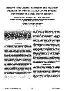
Fig. 3. Comparison of the iterative-channel-estimator performance. perf: with perfect channel knowledge; DA: data aided; DD: decision directed; UEM: unbiased EM; EM 1: one equalizer/decoder iteration per EM iteration; EM 6: 6 equalizer/decoder iterations per EM iteration. 2000 information bits.

Fig. 3 shows the BER for different receivers. Each receiver uses a different channel-estimation algorithm. The curve labelled ‘perf’ corresponds to the performance of the turbo receiver fed with perfect channel knowledge. This curve is a lower bound on the performance of the proposed estimators. The curve labelled ‘DA’ corresponds to the DA estimator. It is only based on the training sequence and therefore is not iterative. At a low BER, the DA-receiver performance is more than 2 dB poorer than the same receiver with perfect parameter knowledge. Assuming that the probabilities p(S|R, Bˆ(n−1) ) in (14) are given by the decoder after convergence, we should wait until convergence of the equalizer/decoder before doing one more EM iteration. This solution is too complex. For the ‘EM 6’ receiver, we assume the convergence is reached after 6 iterations, so there are 6 equalizer/decoder iterations inside one EM iteration. This ‘EM 6’ receiver performs 1 dB better than the DA ML one at a BER ≈ 10−4 . All the other iterative algorithms (‘EM 1’, ‘UEM’, etc.) even use a stronger approximation: they only use one equalizer/decoder iteration per EM iteration. However, the ‘EM 1’ performance is only 0.2 dB poorer than the one of ‘EM 6’. Both ‘EM 1’ and ‘EM 6’ algorithms suffer from the bias (20). That explains their weak performance w.r.t. the UEM and the DD algorithms. The UEM receiver performs 1 dB better than the ‘EM 1’. Although the UEM and the DD curves are close to each other, the DD receiver performance is the best one among the receiver with an embedded channel estimator. At a BER below 5 10−5 , it performs 0.1 dB better than the UEM and is only 0.1 dB away from the ‘perf’ curve. The DD ML algorithm is the best one in Fig. 3. Its complexity per iteration evolves as O(LMs Ls + L3 ) for the channel-tap estimation. In Fig. 4, the DD estimator is compared to its two lower-complexity variants: the DD ML with the “diagonal approxima-

0

10

DA DD DD diag DD ECM

−1

10

−2

BER

10

−3

10

−4

10

−5

10

−6

10

3

4

5

6

Eb/No [dB]

7

8

9

10

Fig. 4. Comparison of the low-complexity estimators w.r.t the DD and the DA estimators. DD diag: DD with the “diagonal approximation”; DD ECM: hard-decision-directed variant of the expectation-conditional-maximization algorithm. 2000 inform. bits. 0

10

DD MMSE

−1

10

−2

BER

10

−3

10

complexity is by far higher than the one of the other considered iterative estimators. V. C ONCLUSION Two new iterative channel-estimation algorithms have been proposed in this paper: the ECM and the MMSE ones. Simulation results show that the turbo-equalization scheme benefits from the iterative refinement of the channel-parameter estimates. All the iterative estimators considered here outperform the classical DA ML method. The performance of several channel-parameter estimators have been compared. It appears that the MMSE one gives very good performance but its complexity is very high. Both UEM and DD receivers perform very closely to the receiver having perfect knowledge of the channel parameters. Both of the low-complexity methods only suffer from a small penalty w.r.t the UEM and the DD receivers. Finally, the EM algorithm is the worst iterative method over the Porat channel, because of the bias of the channel-tap estimate. Future research could be devoted to the robustness of those algorithms to a varying channel. The estimator performance could also be checked in a realistic system with oversampling. R EFERENCES

−4

10

−5

10

−6

10

3

4

5

6

Eb/No [dB]

7

8

9

10

Fig. 5. Comparison of the MMSE and the DD estimators. 200 information bits.

tion” and the DD variant of the ECM. The complexity of both algorithms evolves as O(LMs Ls ). At a BER ≈ 10−5 , the gaps between the DD ML curve and the ‘DD diag’ and ‘DD ECM’ ones are 0.4 and 0.3 dB respectively. There is thus a small loss due to the approximations brought to lower the complexity. However, at a very small cost, both of the approximated DD solutions perform nearly 1.5 dB better than the non-iterative DA ML method. Fig. 5 compares the DD ML receiver to the MMSEbased receiver. The disadvantage of the MMSE channel estimator is its high complexity due to the inversions of the Ms matrices cov{r m , rm }. The size of the matrix cov{r m , rm } is Ls × Ls . For a simulation-time reason, the frame size in Fig. 5 is 200 information bits instead of 2000. Due to this size reduction, the receiver is less efficient. Indeed, the interleaver size is smaller and the number of data symbols to estimate the channel is smaller too. That explains the 3 dB gap between the DD curves in Fig. 3 and 5. At a BER of 2 10−4 , the MMSE curve is 0.5 dB better than the DD one. It seems that the MMSE channel estimator is the best one from the performance point of view but its

[1] A. Glavieux, C. Laot, J. Labat, “Turbo equalization over a frequency selective channel,” Proc. Int. Symp. on Turbo codes and related topics, pp. 96-102, Brest, France, Sep. 1997. [2] H. Meyr, M. Moeneclaey, S. A. Fechtel, “Digital communication receivers: synchronization, channel estimation and signal processing,” Wiley Series in Telecommunications and Signal Processing, USA, 827 p., 1998. [3] C. N. Geoghiades, J. C. Han, “Sequence estimation in the presence of random parameters via the EM algorithm,” IEEE Trans. Commun., vol. 45, pp. 300-308, Mar. 1997. [4] H. Zamiri-Jafarian, S. Pasupathy, “EM-based recursive estimation of channel parameters,” IEEE Trans. Commun., vol. 47, pp. 1297-1302, Sept. 1999. [5] Y. Li, C. N. Geoghiades, G. Huang, “Iterative maximumlikelihood sequence estimation for space-time coded systems,” IEEE Trans. Commun., vol. 49, pp. 948-951, June 2001. [6] M. Kobayashi, J. Boutros, G. Caire, “Successive interference cancellation with SISO decoding and EM channel estimation,” IEEE Journ. on Sel. Areas in Comm., vol. 19, pp. 1450-1460, Aug. 2001. ¨ [7] A. O. Berthet, B. S. Unal, R. Visoz, “Iterative decoding of convolutionally encoded signals over multipath Rayleigh fading channels,” IEEE Journ. on Sel. Areas in Comm., vol. 19, pp. 1729-1743, Sept. 2001. [8] G. Caire, U. Mitra, “Structured multiuser channel estimation for block-synchronous DS/CDMA,” IEEE Trans. Commun., vol. 49, pp. 1605-1617, Sept. 2001. [9] B. Lu, X. Wang, Y. G. Li, “Iterative receivers for space-time block-coded OFDM systems in dispersive fading channels,” IEEE Trans. on Wireless Commun., vol. 1, pp. 213-225, Apr. 2002. [10] R. Otnes, M. T¨uchler, “Soft iterative channel estimation for turbo equalization: comparison of channel estimation algorithms,” in Proc. Intern. Conf. on Communications Systems, Singapore, Nov. 2002. [11] R. Otnes, M. T¨uchler, “On iterative equalization, estimation, and decoding,” in Proc. Intern. Conf. on Communications, Anchorage, USA, May 2003. [12] X. Wautelet, A. Dejonghe, L. Vandendorpe, “MMSE-based Fractional Turbo Receiver with EM Channel Estimation for Space-Time BICM over MIMO Fading Channels,” in Proc. 3rd International Symposium on Turbo Codes & Related Topics, Brest, France, September 1-5, 2003, pp. 519-522.

[13] A. P. Dempster, N. M. Laird, D. B. Rubin, “Maximumlikelihood from incomplete data via the EM algorithm,” J. Roy. Stat. Soc., Ser. B, vol. 39, no. 1, pp. 1-38, Jan 1977. [14] G. Caire, G. Taricco, E. Biglieri, “Bit-interleaved coded modulation,” IEEE Trans. Inform. Theory, vol. 44, pp. 927946, May 1998. [15] M. T¨uchler, A. Singer, R. Koetter, “Minimum mean squared error equalization using a-priori information,” IEEE Trans. on Signal Processing, vol. 50, pp. 673-683, Mar. 2002. [16] L.R. Bahl, J. Cocke, F. Jelinek, J. Raviv, “Optimal decoding of linear codes for minimizing symbol error rate,” IEEE Trans. Inform. Theory, vol. 20, pp. 284-287, Mar. 1974. [17] X. Wautelet, A. Dejonghe, L. Vandendorpe, “MMSEbased Fractional Turbo Receiver for Space-Time BICM over Frequency-Selective MIMO Fading Channels,” IEEE Trans. on Signal Processing, to be published. [18] X. Wang, H. V. Poor, “Iterative (Turbo) soft interference cancellation and decoding for coded CDMA,” IEEE Trans. Commun., vol. 47, pp. 1046-1061, July 1999. [19] C. F. J. Wu, “On the convergence properties of the EM algorithm,” Ann. Statistics, vol. 11, no. 1, pp. 95-103, 1983. [20] G. J. McLachlan, T. Krishnan, “The EM algorithm and extensions,” Wiley Series in Probability and Statistics, USA, 274 p., 1997. [21] J. M. Mendel, “Lessons in estimation theory for signal processing, communications, and control,” Prentice Hall Signal Processing Series, New Jersey, USA, 561 p., 1995.

pressed as: E[ˆ σn2 ] = − = −

M s −1 X

E[(r m − S hm )H (rm − S hm )] Ms Lr m=0 ! H ˆ ˆ − S h )] E[(S hm − S hm ) (S h m m Ms Lr

Ms Lr σn2 (34) Ms Lr M s −1 ˆ − h )H S H S(h ˆ − h )] X E[(h m m m m . M L s r m=0

If the pilot symbols are chosen according to [8], we get: (35) S H S = Lr σs2 I. Since the DA ML channel-tap estimator is efficient, the tap-estimate variance is: ˆ l,m − hl,m )H (h ˆ l,m − hl,m )] = E[(h

The DA ML noise-variance estimate (8) is not biased if the channel taps are known. However, by analogy with the joint estimation of the mean and the variance of a random variable, the ML criterion leads to a biased estimate of σn2 when the noise variance and the channel taps are jointly estimated. Using (7) and the fact that (S H S)H = S H S, it is straightforward to show that: (r m − S hm ) (rm − S hm ) = ˆ )H (r − S h ˆ ) (r − S h m

ˆ − S h )H (S h ˆ − S h ). +(S h m m m m

(33)

With this relation, the expectation of (8) can be ex-

(37)

The bias shown by (37) becomes negligible when Lr >> L. Usually, this is not the case during the acquisition stage because there are only a few pilot symbols. The bias effect is the underestimation of the noise variance. That can lead to convergence problems in the turbo receiver. To avoid the bias, we can use the following unbiased estimate: M s −1 X

1 ˆ )H (r − S h ˆ ). (rm − S h m m m M (L − L) s r m=0 (38) This is the one that is used for the simulations. It has not yet been shown that the EM estimate (17) is biased by the same factor. However, for the simulations, we r the estimates given by (17) or also multiply by LrL−L by (10). σˆn2 =

H

m

σ2 Ms L Lr σs2 n 2 Ms Lr L r σs Lr − L 2 σn . Lr

E[ˆ σn2 ] = σn2 − =

m

(36)

Using the last two relations, (34) becomes:

A PPENDIX

m

σn2 . Lr σs2