pairs of the individual mobile automata in a system, and the external se- mantics are the ..... Invited papers 1: basic concepts of automata theory. In Proc. 20th.
Mobile Automata with External Semantics Dina Q Goldin and Elaine L. Sonderegger Computer Science and Engr. Dept., Univ. of Connecticut, Storrs, CT 06269, USA {dqg,esonderegger}@engr.uconn.edu
Abstract. Mobile automaton (MA) systems are presented as a formal model for emergent behavior in multi-agent systems. A MA system is a group of finite-state transducers moving about, reading, and writing to a shared grid environment. The MAs in a system may be either homogeneous or heterogeneous, and their concurrent system computations may be either synchronous or asynchronous. There is no message-passing among MAs; instead they interact indirectly through the shared values stored in their common grid environment. MA systems are shown to be at least as expressive as cellular automata. We distinguish two ways of characterizing the semantics of a MA system computation; the internal semantics are streams of input/output pairs of the individual mobile automata in a system, and the external semantics are the resulting changes to the contents of the grid environment. Emergent behaviors are formally represented by the external semantics. In the past, understanding the relationship between individual agent behaviors and the resultant emergent behavior of a multi-agent system as a whole has been difficult. It is hoped that the distinction between internal and external semantics, as exemplified by MA systems, will enable the development of effective tools for formalizing emergent computations.
1
Introduction
Computing is becoming increasingly more distributed and mobile. This paper presents mobile automaton systems (MA systems) as a model of simple concurrent and distributed agent computations which exhibit emergent behaviors. A MA system is a group of finite-state automata that move about in a shared grid environment. The behavior of a MA system can be describe both internally as the trace of the states through which each automaton passes during a computation, and externally as the resultant changes in the contents of the grid environment. We begin with the definition of a single mobile automaton in Section 2. Section 3 defines a MA systen and both synchronous and asynchronous system computations. Section 4 demonstrates that a cellular automaton can be simulated with a MA system, and thereby proves that MA systems are at least as expressive as cellular automata. Our principal results begin in Section 5, where we make a distinction between the internal and external semantics of a MA system computation and prove that
2
the external semantics are more expressive than the internal semantics. Section 6 argues that external MA system semantics provide a natural approach for formalizing emergent behaviors. Section 7 compares and contrasts MA systems with several related models, each of which explores the behaviors of multiple computing agents acting in a common grid environment. Section 8 concludes with some suggestions for future work.
2
Mobile Automaton
We begin our formal discussion by defining a single mobile automaton. Definition 1 (Mobile Automaton) A mobile automaton (MA) is a 5-tuple, hid, Q, Σ, δ, F i, where: – – – – –
id ∈ N is an integer identifier. Q is a finite set of states. Σ is a finite alphabet containing the special blank symbol #. δ ⊆ Q × Σ × Q × Σ × {L, R, N}k is the transition relation. F ⊆ Q is the set of final states.
A MA is deterministic if δ is a function δ : Q × Σ → Q × Σ × {L, R, N}k . The direction of the MA’s movement is specified in the transition relation by a k-tuple of direction values corresponding to moving left one cell (L), moving right one cell (R), or not moving (N) in the corresponding dimension of the grid environment. We next define a grid environment. Definition 2 (Grid Environment) A hΣ, G, read, writei, where:
grid
environment
is
a
4-tuple,
– Σ is a finite alphabet containing the special blank symbol #. – G is a k-dimensional semi-infinite grid of cells, each containing a symbol from Σ. – read is a function read : Nk → Σ, which returns the contents of the specified cell in G. – write is an operation write : Nk × Σ, which updates the contents of the specified cell in G using the value in Σ. A grid environment’s read and write operations enable a MA to examine and change the contents of grid cells. The details of these operations are not specified; each grid environment has the flexibility to implement them using the most appropriate shared memory model for its application. Common synchronous models include CREW (concurrent read, exclusive write) and CRCW (concurrent read, concurrent write) [1]. A MA need not have the same dimension as its grid environment. If the dimension of the MA is smaller than the dimension of its grid environment, the
3
behavior of the MA is well-defined, with its movements limited to the smaller dimension of the MA. If, instead, the dimension of the grid environment is smaller than the dimension of the MA, the movement of the MA is limited to the smaller dimension of the grid environment. For the remainder of this paper, we assume the dimension of the MA and the dimension of the grid environment are the same. A MA computes by interacting with its grid environment, repeatedly performing a series of steps. For MA M in state q at position p in grid environment E, the steps are: 1. M asks E for the contents of the grid cell at p using E’s read operation, denoted E.read(p). Let x be the value returned by E.read(p). 2. M finds an appropriate tuple, hq, x, q 0 , x0 , di ∈ δ, corresponding to q and x. 3. M asks E to write x0 at p, denoted E.write(p, x0 ). 4. M updates its state to q 0 . 5. M moves to a new position p0 as prescribed by d. We call this series of steps a transition and the associated input/output pair, x/(x0 , d), an action. Definition 3 (Transition) Let M be a MA with states q, q 0 ∈ Q and positions p, p0 ∈ Nk within a k-dimensional grid environment E. Let p = hp1 , . . . , pk i and p0 = hp01 , . . . , p0k i. A transition of M in state q and position p is a movement to state q 0 and position p0 and an invocation of E.write(p, x0 ), denoted hq, pi 7→ hq 0 , p0 i, where hq, E.read(p), q 0 , x0 , hd1 , . . . , dk ii ∈ δ and for i = 1, . . . , k: p0i = pi + 1 if di = R p0i = pi − 1 if di = L and pi 6= 1 p0i = pi otherwise Definition 4 (Action) Let M be a MA, and let hq, pi 7→ hq 0 , p0 i be a transition of M corresponding to hq, x, q 0 , x0 , di ∈ δ. The action associated with hq, pi 7→ x/(x0 ,d)
hq 0 , p0 i is the input/output pair, x/(x0 , d), and may be denoted as hq, pi 7−→ hq 0 , p0 i.
Now we can define a mobile automaton computation as a sequence of transitions. Definition 5 (Mobile Automaton Computation) Let M be a MA in some initial state q0 ∈ Q and position p0 ∈ Nk . A mobile automaton computation is a sequence of transitions hq0 , p0 i 7→ hq1 , p1 i 7→ . . . 7→ hqn−1 , pn−1 i 7→ hqn , pn i for some n > 0 with qn ∈ F . Example 1 Consider a two-dimensional MA MLines with alphabet {W hite, Gray, Black} and states {Across, Down} that moves about in its environment in straight lines. If the MA is in a white cell, it stores gray in that cell; otherwise it leaves the contents of the cell unchanged, changes its direction from horizontal to vertical or vice versa, and continues its journey. Figure 1 shows the transition diagram and one computation of MLines . Within the transition diagram,
4
“W/G, hR, N i” is shorthand for the action that when reading White, MLines writes Gray and moves one cell to the right. The grid environment initially is mostly white with some randomly placed black cells, and MLines initially is near the top left-hand corner.
G/G, B/B, Across W/G,
Down G/G,
W/G,
B/B,
Fig. 1. Transition diagram and one computation of MLines
3
Mobile Automaton System
A mobile automaton system is a group of MAs moving about in a shared grid environment. Definition 6 (Mobile Automaton System) A mobile automaton system is a pair, hE, Mi, where: – E is a grid environment with alphabet Σ. – M is a set of mobile automata Mi = hidi , Qi , Σ, δi , Fi i, with idi = idj ⇐⇒ Mi = Mj . A MA system is simple if it has only one MA and uniform if all of the MAs have the same transition relation. Next, we introduce a configuration, which is an instantaneous description of a MA system. A configuration captures both the location of each MA in the system’s grid environment and the contents of each grid cell. Note there is no restriction on the number of MAs that can be positioned simultaneously in a single grid cell. Definition 7 (Configuration) Let S = hE, Mi be a MA system. A configuration of S is a pair, hP, Xi, where:
5
– P is a set of triples, hidi , qi , pi i, with one triple for each MA Mi ∈ M. Within each triple, idi ∈ N is the identifier of Mi , qi ∈ Qi is the current state of Mi , and pi ∈ Nk is the current position of Mi in E. – X is a k-dimensional, possibly infinite, array of symbols in Σ, corresponding to the current contents of each cell in E. An initial configuration of S is any configuration that specifies both the initial position and initial state for every Mi ∈ M and the initial contents of E. A final configuration of S is any configuration with qi ∈ Fi for every tuple hi, qi , pi i ∈ P . The behavior of a MA system can be either synchronous or asynchronous. This distinction between synchronous and asynchronous refers to system transitions, not communications as in [2]. Each asynchronous transition involves the movement of a single MA from one configuration to the next, whereas each synchronous transition involves the simultaneous movement of all of the MAs in the system. In the synchronous case, if multiple MAs simultaneously try to write to the same grid cell, the conflict is resolved by the shared write operation of the grid environment. This is stated more formally in the following definitions. Definition 8 (Asynchronous System Transition) Let S be a MA system and C, C 0 be two configurations of S, with C = hP, Xi and C 0 = hP 0 , X 0 i. We say that a C 7→ C 0 ( yields in one asynchronous system transition) if for exactly one MA Mi in S, there exist hidi , qi , pi i ∈ P and hidi , qi0 , p0i i ∈ P 0 such that hqi , pi i 7→ hqi0 , p0i i. For all other MAs Mj in S with i 6= j, hidj , qj , pj i ∈ P ⇐⇒ hidj , qj , pj i ∈ P 0 . Definition 9 (Synchronous System Transition) Let S be a MA system and C, C 0 be two configurations of S, with C = hP, Xi and C 0 = hP 0 , X 0 i. We say s that C 7→ C 0 ( yields in one synchronous system transition) if for every MA Mi in S, there exist hidi , qi , pi i ∈ P and hidi , qi0 , p0i i ∈ P 0 such that hqi , pi i 7→ hqi0 , p0i i. During both synchronous and asynchronous system transitions, the MAs involved in the system transition invoke the grid environment’s write operation to effect changes to the contents of the grid environment. Such changes in the contents of the system’s grid environment are called an environment transformations, and correspond to the “external” computational semantics of a MA system. Definition 10 (Environment Transformation) An environment transition t of a MA system S is a relation between the contents of S’s grid environment before and after a synchronous or asynchronous system transition, i.e. s a t(X, X 0 ) ⇐⇒ hP, Xi 7→ hP 0 , X 0 i or hP, Xi 7→ hP 0 , X 0 i where hP, Xi and hP 0 , X 0 i are configurations of S. An environment transformation T is the transitive closure of t. The external semantics for an initial configuration C0 = hP0 , X0 i of S is the set of all X such that T (X0 , X). A system computation begins with some initial configuration and proceeds, with system transitions from one configuration to the next, until the system is
6
in a final configuration with each of the MAs in the system in a final state. A system computation can be either synchronous or asynchronous, depending upon whether the system transitions are synchronous or asynchronous. If the system transitions are asynchronous, the system must exhibit fairness, ensuring that every MA in the system eventually gets a chance to move [3]. If the system transitions are synchronous, the MAs in the system may not enter a final state at the same time; in that case the system computation continues with the just the active MAs. Definition 11 (System Computation) Let S be a MA system and C0 be an initial configuration of S. An asynchronous system computation is a sequence a a of asynchronous system transitions C0 7→ C1 , . . . , Cn−1 7→ Cn for some n > 0 and Cn a final configuration of S. Similarly, a synchronous system computation s s is a sequence of synchronous system transitions C0 7→ C1 , . . . , Cn−1 7→ Cn for some n > 0 and Cn a final configuration of S. MAs communicate with each other by writing values in a shared grid environment. More specifically, each MA leaves data behind in the grid environment for other MAs to discover at later times. This type of communication is known as indirect interaction [4, 5], and can be contrasted with direct interaction techniques such as message passing. Example 2 Consider a two-dimensional MA system SLines beginning with a white grid environment and an assortment of MAs similar to MLines from Example 1. Half of the MAs in SLines write in gray, and half write in black; some move across and down like MLines , and some move in each of the other three directions. Each MAs changes direction any time it visits a gray or black cell, i.e. one that was previously visited by another MA. If SLines ’s computation is synchronous, the MAs always cross paths at the same locations and the resulting environment transformation is deterministic. However, if SLines ’s computation is asynchronous, the locations where the MA cross paths and the resulting environment transformation are nondeterministic. Figure 2 shows the environment transformations for two asynchronous computations of SLines , each beginning with the same initial configuration of MAs. Example 2 shows that when the MAs in a system interact and the system computations are asynchronous, nondeterministic behaviors may result. This may occur even if each of the MAs are deterministic. The nondeterminism results from the differences in speed of the individual MA computations. Note that both the synchronous and asynchronous system computations are deterministic if there are no interactions among the MAs, e.g. if all the MAs in SLines only write gray and only turn on black or if there is only one MA in the system.
4
Simulation of Cellular Automata
Much research has been devoted to cellular automata; for an overview see [6]. A simple cellular automaton is a k-dimensional array of cells, each of which is in
7
Fig. 2. Two asynchronous computations of SLines , each beginning with the same configuration
one of a finite set of states. Every clock tick all the cells synchronously transition to new states, where each cell’s new state depends only on its current state and the states of its immediate neighbors. There is no input other than the initial configuration and no output. Cellular automata exhibit surprisingly complex behaviors. A cellular automaton can be simulated with a uniform MA system with one MA at each grid location, where the initial contents of the grid environment are the initial cell states of the cellular automaton. The MA system uses synchronous system transitions; for each cellular automaton step, the following system transitions are required: – Each MA visits each of its neighboring grid cells, reading the contents of the grid environment at each of those locations. – Each MA remembers the contents of its neighboring cells using its internal states. Both the alphabet of the cellular automaton and the number of its neighbors are finite, so only a finite number of MA states are required. – Each MA returns to its “home” cell and writes the value specified by the cellular automaton’s rule to its grid cell. After each simulation step, the contents of the grid environment correspond to the cell states of the cellular automaton. Theorem 1 (Cellular Automata Expressiveness) The external semantics of uniform MA systems are at least as expressive as cellular automata. Proof. (outline) Cellular automata can be simulated by uniform MA systems, as above. Traditional cellular automata have a deterministic rule, with each cell using the same rule. Many variations of cellular automata also have been studied, as summarized in [6]. These include cellular automata with nondeterministic rules,
8
cellular automata where each cell has its own rule, cellular automata with only one-sided neighborhoods, and asynchronous cellular automata. It appears that MA systems can be used to simulate these variations of cellular automata as well; we will study these as future work.
5
Internal versus External Behaviors
There are two ways to view the behavior of a MA system, internally and externally. Internally, each of the MAs in a system makes a series of state transitions in response to the values it reads from the environment, along the way outputting new values to the environment and moving to new positions. Externally, the MAs make a series of changes in the contents of the grid environment in response to the values read from the environment. In this section we investigate the differences between these two views of MA behavior. We begin by defining the two types of behaviors more carefully. Definition 12 (Internal Behavior) The internal behavior of a MA system is the sequence of actions (Definition 4) associated with a system computation. Definition 13 (External Behavior) The external behavior of a MA system is the sequence of environment transitions (Definition 10) associated with a system computation. To understand the differences between these two behaviors, consider a MA system with a single MA moving around in a one-dimensional grid environment. Viewed internally, this MA system behaves like a finite state transducer, repeatedly getting an input symbol from its environment, updating its state accordingly, and outputting a symbol to its environment; its output alphabet consists of pairs of input symbols and direction values. In contrast when viewed externally, this MA system behaves like a Turing machine, repeatedly reading a symbol from its tape (the one-dimensional grid environment), updating its state accordingly, writing a new symbol on its tape, and moving to an adjacent cell. We first show that the internal behavior of this MA system corresponds to the behavior of a finite-state transducer. Theorem 2 (Transducer Correspondence) The internal behavior of a simple MA system corresponds exactly to the behavior of a finite-state transducer. Proof. Let S be a simple MA system, and let M = hid, Q, Σ, δ, F i be the single MA in S, with M initially in state q0 ∈ Q. The corresponding finite-state transducer is T = hQ, Σ, (Σ × {L, R, N}k ), δ, q0 , Fi, where Q is the finite set of states, Σ is the input alphabet, (Σ × {L, R, N}k ) is the output alphabet, δ is the transition relation, q0 ∈ Q is the initial state, and F ⊆ Q is the set of final states. We next show that the external behavior of this MA system corresponds to the behavior of a single-tape Turing machine.
9
Theorem 3 (Turing Machine Correspondence) The external behavior of a one-dimensional simple MA system corresponds exactly to the behavior of a single-tape Turing machine. Proof. Let S be a one-dimensional simple MA system, and let M = hid, Q, Σ, δ, F i be the single MA in S. Let the initial system configuration have M in state q0 ∈ Q, positioned in the leftmost cell of the one-dimensional grid environment E. The corresponding single-tape Turing machine is T M = hQ, Σ, δ, q0 , F i, where Q is the finite set of states, Σ is the tape alphabet, δ is the transition relation, q0 ∈ Q is the initial state, and F ⊆ Q is the set of final states. Corollary 1 (Expressiveness) The external behavior of a one-dimensional simple MA system is more expressive than its internal behavior. Proof. Turing machine computations are more expressive than finite-state transducer computations [7]. For a MA system with more than one MA, the external behavior is still a sequence of environment transitions, but the internal behavior is now characterized by a set of transducer streams. For Example 2, the internal behavior is the set of streams of colors read, colors written, and movements of the individual MAs in the system such as {W/G, hR, N i, W/G, hR, N i, B/B, hN, Ri, . . .}, and the external behavior is the sequence of patterns of white, gray, and black cells. Corollary 1 presents a paradox: the expressiveness of a simple MA system varies, depending upon whether its behavior is viewed internally or externally. A simpler machine, e.g., a finite-state transducer, becomes equivalent to a more powerful machine, e.g., a Turing machine, when it interacts with its environment. Greater expressiveness comes from focusing on the environment transformations emerging from MA system computations, rather than focusing on the traces of actions used to produce those transformations. What is the source of this greater expressiveness? It appears to be a result of an “entanglement” of input and output. A MA can read the contents of a grid cell that it has previously written, or has been written by another MA in the system. Similarly, a Turing machine can read the contents of a cell it has previously written. In fact, a Turing machine that can only move forward, but not backward, is not as expressive as a Turing machine that can reread its output; it needs an entanglement of input and output to achieve its full expressiveness. For a MA system, the grid environment provides the capability for this entanglement. The internal and external semantics are two different ways to characterize the behavior of exactly the same MA system. The internal semantics correspond to the traditional view of multi-agent systems, whereas the external semantics are more appropriate for modeling emergent behaviors (Section 6).
6
Emergent Computation
The classic example of emergent behavior is ants collectively foraging for food; each ant, by leaving behind pheromone when it returns to the nest with food,
10
helps form an emergent pheromone-based “ant highway” that other ants follow directly to the food source. However, there is no widespread agreement on what constitutes an emergent computation. For many, emergent computation refers to the global information-processing capabilities that appear to emerge from local interactions among simple component parts [8, 9]. Ronald, Sipper, and Capcarr`ere [10] have formulated an emergence test which they call “design, observation, surprise”. According to their test, a system exhibits emergence if an observer is “surprised” because he cannot reconcile the observed global behavior of the system with his knowledge of the elementary interactions. Kub´ık [11] prefers to define emergence as “a property of the system that can be produced by interactions of its agents (components) with each other and with the environment and cannot be produced by summing behaviors of individual agents in the environment”. Kub´ık notes that each “agent acts autonomously in order to fulfill its internal goals.” The emergent behaviors are a result of the inherent parallelism of the agents’ interactions. MA systems provide a natural model for computing systems that exhibit emergent behavior. The individual MAs in a system correspond to the simple component parts, and the changes to the grid environment correspond to the observed global behavior, or external semantics, of the computation. Inter-agent interactions are modeled by MAs reading grid cells that were previously written by other MAs. The interactions are indirect and may be both parallel and nondeterministic. As in Example 2, emergent behaviors may result as a system computation proceeds. Claim 1 (Emergent) The behavior of a MA system is emergent. Previous efforts to formalize global emergent behaviors have focused on formalizing the internal behaviors of the individual components. We have shown that these two levels of behaviors do not have the same expressiveness (Corollary 1 in Section 5). Therefore, the formalization of emergent behaviors must be on the external semantics level instead. MA systems, by making this distinction between internal and external semantics, will enable more substantial progress to be made in understanding the foundations of emergence.
7
Related Work
MA systems offer a unifying model which combines the best of both cellular automata and simple multi-agent (swarm) systems. The fields of artificial life and swarm intelligence [12, 13] have seen many approaches to multi-agent computation somewhat similar to ours, including blob computing [14], amorphous computing [15, 16], and StarLogo [17]. We view our work as part of the models of computation community instead, with the goal of studying the expressiveness of external vs. internal semantics, specifically for emergent behaviors.
11
In a similar spirit, Wiedermann and van Leeuwen [18] have investigated finitestate transducers that move about in a shared environment. Their “active cognitive transducers” are similar to mobile automata, but they communicate both by sending messages and writing to environment. Their transducers also are “mortal”, emerging and vanishing unpredictably. It was shown that communities of active cognitive transducers are equivalent to Turing machines with advice. By contrast, our model is much simpler, representing a minimal extension of finitestate transducers to mobility and concurrency, and relying exclusively on indirect interact for communication. An analogous difference in expressiveness between the external and internal semantics of a model of computation can also be observed for Persistent Turing Machines (PTMs), a sequential interactive model that extends Turing machines with dynamic stream semantics and persistence [19]. The internal semantics of PTMs are those of Turing machines, but the external semantics are more expressive as proven in [19]. Individual PTMs do not exhibit emergent behavior, due to their sequential nature. Furthermore, not all systems of independent interacting components result in emergent behavior. For example, Doyle and Kalish [20] report that their model of robots moving blocks did not result in emergent behavior because the robot motions could be modeled as sequential, rather than parallel, actions.
8
Future Work and Conclusions
We have presented MA systems as a model for studying emergent behaviors in multi-agent systems. We have shown that MA systems are at least as expressive as a cellular automata. The behavior of a MA system can be viewed in two ways, focusing either on the internal semantics of each MA computation or on the external semantics of the system computation as a whole. There is a difference in expressiveness between these two views. We believe this distinction between internal and external semantics is central to an understanding of emergent computation. Several extensions to the MA system model are being considered. First, we would like to explore the implications of an open, rather than a closed, system of MAs, where individual MAs can be added to the system or deleted from the system in the middle of a system computation. This is similar to the “mortal” transducers in Wiedermann and van Leeuwen’s communities [18] and the unreliable components in amorphous computing [15]. Second, the movements of individual MAs may be expanded to include movements of more than one unit in each dimension, or possibly continuous movements. The movements also may be decoupled from the MAs and become an operation of the environment, thereby allowing the environment to factor in forces such as wind and friction in determining updated positions. We have just scratched the surface on expressiveness results for MA systems. Several extensions to the cellular automata result were suggested at the end of Section 4. Another area that should be explored is the differences in expres-
12
siveness, if any, between synchronous and asynchronous systems. It is hoped that such a study will yield a better understanding of the roles parallelism and nondeterminism play in emergent behavior.
References 1. P. C. Kanellakis and A. A. Shvartsman. Fault-Tolerant Parallel Computation. Kluwer Academic Publishers, Norwell, MA, 1997. 2. C. Palamidessi. Comparing the expressive power of the synchronous and the asynchronous pi-calculus. Math. Structures in Computer Science, 13(5):685–719, 2003. 3. N. Francez. Fairness. Springer-Verlag, New York, 1986. 4. D. Keil and D. Goldin. Modeling indirect interaction in open computational systems. WETICE 2003, IEEE Press, 2003. 5. D. Goldin and D. Keil. Toward domain-independent formalization of indirect interaction. WETICE 2004, IEEE Press, 2004. 6. P. Sarkar. A brief history of cellular automata. ACM Comp. Surveys, 32(1), Mar 2000. 7. R. J. Nelson. Invited papers 1: basic concepts of automata theory. In Proc. 20th Nat’l Conf., pages 138–161. ACM Press, 1965. 8. S. Forrest. Emergent computation: self-organizing, collective, and cooperative phenomena in natural and artificial computing networks. In Emergent computation. MIT Press, 1991. 9. J. P. Crutchfield and M. Mitchell. The evolution of emergent computation. Proc. of the National Academy of Sciences, 92(23), 1995. 10. E. M.A. Ronald, M. Sipper, and M. S. Capcarr`ere. Design, observation, surprise! a test of emergence. Artificial Life, 5(3):225–239, 1999. 11. A. Kub´ık. Toward a formalization of emergence. Artificial Life, 9(1):41–65, 2003. 12. P. Tarasewich and P. R. McMullen. Swarm intelligence: power in numbers. Comm. of the ACM, 45(8):62–67, 2002. 13. E. Bonabeau, M. Dorigo, and G. Theraulaz. From Natural to Artificial Swarm Intelligence. Oxford University Press, 1999. 14. F. Gruau, Y. Lhuillier, P. Reitz, and O. Temam. Blob computing. In Proc. 1st Conf. on Computing Frontiers. ACM Press, Apr 2004. 15. H. Abelson, D. Allen, D. Coore, C. Hanson, G. Homsy, Jr. T. F. Knight, R. Nagpal, E. Rauch, G. J. Sussman, and R. Weiss. Amorphous computing. Comm. of the ACM, 43(5), May 2000. 16. D. Servat and A. Drogoul. Combining amorphous computing and reactive agentbased systems: a paradigm for pervasive intelligence? In Proc. 1st int’l joint conf. on Autonomous agents and multiagent systems, pages 441–448. ACM Press, 2002. 17. M. Resnick. Turtles, Termites, and Traffic Jams: Explorations in Massively Parallel Microworlds. MIT Press, Cambridge, MA, 1994. 18. J. Wiedermann and J. van Leeuwen. The emergent computational potential of evolving artificial living systems. AI Comm., 15(4):205–215, 2002. 19. D. Q. Goldin, S. A. Smolka, P. C. Attie, and E. L. Sonderegger. Turing machines, transition systems, and interaction. Information & Computation, 194(2), Nov 2004. 20. M. Doyle and M. Kalish. Stigmergy: Indirect communication in multiple mobile autonomous agents. In M. Pechoucek and A. Tate, editors, Knowledge Systems for Coalition Operation, pages 151–158. Czech Technical University, Prague, 2004.