Adaptive Automata for Mobile Robotic Mapping Miguel Angelo de Abreu de Sousa
[email protected]
André Riyuiti Hirakawa
[email protected]
João José Neto
[email protected]
Escola Politécnica da Universidade de São Paulo Departamento de Engenharia de Computação e Sistemas Digitais Av. Prof. Luciano Gualberto, travessa 3, nº 158. São Paulo - SP - Brasil - CEP 05508-900 Abstract Robotic mapping deals with the question of building abstract representation of the physical environment around a mobile robot and it is one the most important features of a truly autonomous mobile robot. This work presents an adaptive way to make such representation without a priori knowledge of the environment. Starting with a small net and through simple reconfiguration rules, this net is expanded by acquiring the map of the place while the robot travels. The initial configuration contains free marks, which are replaced with information acquired by the sensors. This paper also presents an adaptive algorithm for exploring motion.
1. Introduction Early approaches for solving the motion problem in mobile robots used to employ a preliminary map of the environment stored in the robot’s memory. Such approach presents three main problems [2]: the first one refers to its computational complexity. Storing a complete geometrical map of the environment, searching the database for localization and path planning process increase the computational complexity. This problem makes this approach prohibitive for real implementations. The second question is related to the requirement of repetitive task of the non-automatic mapping process before the robot’s work in a variety of unstructured environments. Each house, factory, street, office, hotel, hospital and agricultural field where the robot is intended to work has to be mapped and the resulting map must be manually registered in its memory. Finally, robots may have to work in unknown and hazardous environments. Mining, undersea operations, working in disaster areas, space and planetary exploration are examples of possible tasks in which robots have to map the field before being able to work properly.
Due to those reasons, robotic mapping has been a strongly researched topic in robotics and artificial intelligence for two decades and is still an interesting research subject. For instance, the mapping process of dynamic or large areas is still challenging [9]. The present work employs an adaptive mechanism to collect information from the environment and organize this information as a map for further use in navigation. Adaptive automata, proposed by [7], are able to reconfigure themselves. Consequently, their behavior may be changed according to externally collected information. In this mapping application, adaptive automata start from a simple initial model, and change their structure according to the properties of the field around. The adaptive feature allows the proposed mechanism to map the environment without a priori knowledge of the place and also allows memory space occupied just grows up accordingly to the already mapped area. Such adaptability represents an intuitive and trustful way for modeling the physical environment during the robot’s motion. The following section briefly reviews previous works in the area. Section 3 sketches the adopted formalism. Section 4 presents the system, which includes the exploring motion automaton and the mapping automaton. Sections 5 and 6 describe details of the implementation of the automata for this application. Finally, the last two sections describe simulation results, conclusions and future works.
2. Related Work Since the early 80’s robotic mapping research area was conducted by using two approaches, namely, topological and metrical. While metric maps represent the environment by using its geometric properties [4] [8], topological ones describe environments by expressing the connectivity of their distinct spaces [2] [6]. Nevertheless, the exact frontier between these approaches has never been clearly stated, since
topological maps rely on geometric information about the world [9]. This paper describes some interesting results achieved by extending a previous work on the representation of physical environments by using adaptive automata [5]. Adaptive automata’s learning capability is due to their reconfigurable behavior, turning them suitable for representing knowledge and for implementing learning features. It has been shown that adaptive automata are Turing-powerful devices [7], which allow the system to store and handle gathered information by using rather simple rules. Adaptive devices have also been applied in several other applications, such as pattern recognition [3] and systems description [1].
A graphic representation of the transition is the following:
3. Adaptive Automata
4. The Model
Adaptive automata may be viewed as self-modifying state machines whose structure includes a set of states and a set of transitions interconnecting such states. States may be classified in: initial state (S); a set of final states (F); and a set of intermediate states. Incoming stimuli change the internal state of the machine. The self-modifying feature of adaptive automata is due to the capability it has of changing its own set of transition rules. Adaptive actions may be attached to the transitions which are able to either add new states and transitions or remove already existents ones, consequently, achieving a new structure. Hence, incoming stimuli may change the set of internal states and modify the general configuration of the automaton. See [7] for details on concepts and notation. Transition rules in adaptive automata are represented as:
The present paper describes the proposal of modeling robotic mapping and exploring motion by the use of adaptive automata. The model proposed is depicted in figure 2:
e
a B. , .A
e'
Figure 1. Adaptive automata transition.
Adaptive actions A and B are both optional. Three different elementary adaptive actions are allowed: inspection – search the current state set for a given transition; deletion – erase a given transition from the current state set; and insertion – add a given transition to the current set of states. Such actions are denoted by preceding the desired transition by the signs ?, – and +, respectively.
Sensors Obstacle information
Sensor and motion information
Exploring motion automaton
Mapping automaton
Border information
Motion
( g , e , a ) : B → ( g’ , e’ , a’ ) : A g: push-down store contents before the transition; g’: push-down store contents after the transition; e: current state before the transition; e’: current state after the transition; a: input stimulus before the transition; a’: input stimulus after the transition; B: adaptive action before applying the transition; A: adaptive action after applying the transition. Whenever g, g’ and a’ are all omitted, the representation may be simplified to: ( e , a ) : B → e’ : A
Motion system Figure 2. System model.
In this proposal, an information management system receives data from the sensors and transfers preprocessed information to the exploring motion automaton, which is designed to make decisions on the next move to be performed by the robot. Such decisions are based on: data coming from the sensors; the current neighborhood information extracted from the mapping subsystem; and the motion-controlling algorithm. The motion decision is transferred both to
the motion system that controls the actual motors and to the mapping automaton. The mapping subsystem is responsible to store all the sensor information on the presence or absence of obstacles close to the robot during its travel. The current environment place corresponds to the current state in the mapping automaton.
5. The Mapping Automaton
Once the automaton is supplied with the four-data information collected by the robot’s sensors while it performs its exploring motions, the four adjacent nonfilled transitions are properly replaced according to that information (see figure 5). The information collected by the sensors contain indications on the direction – north (N), south (S), east (E) or west (W) – and condition – free or busy. Double arrows indicate nonobstructed areas and bold lines denote obstructed ways.
The proposed method for the adaptive robotic mapping starts from a square lattice (see figure 3) consisting of nine nodes connected by special transitions denoting areas yet to be mapped (represented by the states and transitions of an adaptive automaton). The central state is the initial state of the automaton, and represents the starting point of the robot’s exploring path. In order to allow a clear presentation of the method, a graphic representation of the adaptive automaton will be used, as described in section 3.
Figure 3. Initial lattice in an adaptive automaton.
The dot-marked state ( ) corresponds to the actual position of the robot and single lines represent areas not yet mapped. In order to complete the representation of the initial automaton, special tags (X) mark corner states, and special transitions are provided for supporting expansions in the lattice as shown in figure 4.
Figure 5. The 16 possible information collected by the sensors.
Figure 4. Complete initial automaton lattice.
Following the information collected by the sensors, the exploring automaton supplies the mapping automaton with the next move to be performed by the robot. Such move may be N, S, E or W and is conditioned to the availability of some appropriate free way in the lattice. As the robot moves (such occurrence is represented by some consistent state change in the
automaton), the current lattice is expanded in the direction of the move. This expansion is performed by adding of a line or a column to the existent lattice. Figure 6 exemplifies the result of an N-move, after reconfiguring the vacant marks corresponding to all free directions.
Figure 6. Expanded lattice after an N-move.
Concluding the changing operation, adaptive actions set new marks to the vertex nodes in the lattice and new auxiliary transitions supporting lattice expansions as shown in figure 7 (note that figure 7 shows a similar configuration to the figure 4 but contains registered some information about the place):
follows the wall until it finds another corner. Then, it turns around and comes back in a parallel way. Such adaptive automaton may be textually described as follows (note that most transitions are similar to finite-state automata’s, but they call functions A, B, C and D. So they constitute adaptive transitions performing the corresponding adaptive actions, described ahead): S = 3; P={ (3,n) →5, (4,s) →7, (6,d) →9, (9,m) →9, (9,p) →9, (8,f) →10, (10,t) →10, (10,q) →10:B(10), (11,p) →11, (7,c) →7, (7,f) →12, (12,p) →12, (7,m) →13, (13,p) →13, (5,b) →5, (5,d) →5, (5,t) →14, (14,v) →14:C(14), (15,p) →15, (10,u) →16, (12,u) →18, (13,u) →20,
F = { 22 }; (3,a) →4, (4,b) →6, (6,c) →6, (6,o) →8, (9,g) →9, (9,v) →9:A(9), (8,m) →11, (10,p) →10, (11,g) →11, (11,q) →11:A(11), (7,o) →7, (12,g) →12, (12,q) →12:B(12), (13,g) →13, (13,q) →13:C(13), (5,c) →5, (5,f) →5, (14,p) →14, (5,g) →15, (15,v) →15:A(15), (16,q) →17:B(17), (18,q) →19:B(19), (20,q) →21:D(21)}
The modifications performed by the adaptive actions A, B, C and D are described as follows:
Figure 7. Operation completed.
6. The Exploring-Motion Automaton An adaptive automaton is used for determining the robot’s next move. For this purpose, it is supplied with information collected by the sensors and with neighborhood information previously modeled in the map. Its operation allows the robot to cover the entire environment by describing a zigzag path: starting in a corner of the environment, for instance, the robot
A(e){: +[(e,#) →22] +[(1,S) →2]}
B(e){: +[(e,#) →22] +[(1,N) →2]}
C(e){: +[(e,#) →22] +[(1,E) →2]}
D(e){: +[(e,#) →22] +[(1,W) →2]}
The output information generated by this automaton indicates in which direction – north (N), south (S), east (E) or west (W) – the robot is going to move. The manager system supplies the mapping automata with the information collected from sensors followed by this direction information.
7. Simulation Simulations of the environment, sensors and motion have been implemented in order to validate the proposed map-building mechanism. Figure 8 shows one of such artificial environments created for this experiment. The initial configuration of the mapping automaton has been presented in figure 3 and contains no information on the environment. The final configuration is presented in figure 9. Such configuration is reached after the robot had completed all the path imposed by the exploring motion automaton and after the mapping automaton expanded the initial lattice modeling the characteristics of the environment, i.e., mapping. The robot is initially placed in the leftmost upper square in the simulator (identified as ‘X’ marked cell in figure 8) and the exploring motion automaton directs it until the rightmost upper square (identified with the dot-marked state ( ) in figure 9). Hence, as presented in figure 9, the memory space used to store the maps acquired in the present work increases with the actual mapped area. Note that in this arrangement the memory space required is proportional to the product of the maximum vertical variation by the maximum horizontal variation of space already visited.
8. Conclusion and Future Work Robotic mapping is an important process for getting truly mobile robots and is also an essential feature to allow robots to complete certain tasks in unstructured and unknown environments. This work has shown an alternative to the classic mapping approaches: adaptive algorithms provide a new way to build such map. A lattice-shaped adaptive automaton grows dynamically in response to the robot’s motion. Sensors attached to the robot scan the environment for the presence or absence of close obstacles, and such information is collected into the model by enabling the automaton to perform appropriate self-modifications. The present proposal has the advantage of building a map without a priori knowledge of the environment and the use of memory space increases with the actually mapped area. These features contrast with some classic approaches (e.g., [4], [6], [10]). Future works should deal with optimizing the representation of the working segment in the acquired map, approaching the navigation problem by using the optimized map segment and handling dynamic
obstacles by exploring the adaptive feature of the formalism.
10. References [1] Almeida Jr., J. R.; Neto, J. J. “Using Adaptive Models for Systems Description, Applied Modelling and Simulation”, International Conference on Applied Modelling and Simulation, Cairns, Australia, 1999. [2] Brooks, R. A. “Visual Map Making for a Mobile Robot”, Proceedings IEEE International Conference Robotics and Automation., St. Louis, MO, 1985, pp. 824–829. [3] Costa, E. R.; Hirakawa, A. R.; Neto, J. J. “An Adaptive Alternative for Syntactic Pattern Recognition”, Proceeding of 3rd International Symposium on Robotics and Automation, ISRA 2002, Toluca, Mexico, 2002, pp. 409413. [4] Donald, B. R.; Howell J. “Practical Mobile Robot SelfLocalization”, Proceedings International Conference on Robotics and Automation, San Francisco, CA, 2000. [5] Hirakawa, A. R; Júnior, J. R. A.; Neto, J. J. “Adaptive Automata for Independent Autonomous Navigation in Unknown Environment”, International Conference on Applied Simulation and Modelling, Banff, Alberta, 2000. [6] Jennings, J.; Kirkwood-Watts, C.; Tanis, C. “Distributed Map-Making and Navigation in Dynamic Environments”, 1998. [7] Neto, J. J. “Adaptive Automata for Context-Dependent Languages”, ACM SIGPLAN Notices, 1994, v.29, n.9, pp.115-24. [8] Sukhatme, G. S.; Wolf, D. F. “Towards Mapping Dynamic Environments”, Proceedings of the International Conference on Advanced Robotics, 2003, pp. 594-600. [9] Thrun, S. “Robotic Mapping: A Survey”, Exploring Artificial Intelligence in the New Millenium, Morgan Kaufmann, 2002. [10] Zimmer, U. R. “Embedding local map patches in a globally consistent topological map”, Proceedings of the International Symposium on Underwater Technology, Tokyo, Japan, 2000, pp.301-305.
Figure 8. Environment simulated using a software tool (the big arrow indicates the initial square).
Figure 9. The lattice modeled by the mapping automaton (the big arrow indicates the final state).