Robotics and Autonomous Systems 34 (2001) 117–129
Mobile robot self-localisation using occupancy histograms and a mixture of Gaussian location hypotheses夽 Tom Duckett a,∗,1 , Ulrich Nehmzow b,2 a
Centre for Applied Autonomous Sensor Systems, Department of Technology, University of Örebro, S-70182 Örebro, Sweden b Department of Computer Science, University of Manchester, Manchester M13 9PL, UK
Abstract The topic of mobile robot self-localisation is often divided into the sub-problems of global localisation and position tracking. Both are now well understood individually, but few mobile robots can deal simultaneously with the two problems in large, complex environments. In this paper, we present a unified approach to global localisation and position tracking which is based on a topological map augmented with metric information. This method combines a new scan matching technique, using histograms extracted from local occupancy grids, with an efficient algorithm for tracking multiple location hypotheses over time. The method was validated with experiments in a series of real world environments, including its integration into a complete navigating robot. The results show that the robot can localise itself reliably in large, indoor environments using minimal computational resources. © 2001 Elsevier Science B.V. All rights reserved. Keywords: Mobile robot navigation; Place recognition; Occupancy grids; Multiple hypothesis tracking; State estimation; Kalman filtering
1. Introduction Perhaps the most fundamental competence required for navigation by a mobile robot is that of self-localisation (location recognition). A wide variety of localisation methods have been proposed, and a number of successful laboratory prototypes have been developed [2]. Some of these systems have been validated in larger environments, generally consisting of enclosed areas within public buildings (Section 1.1). 夽 A major part of this work was carried out for the principal author’s Ph.D. Thesis at the University of Manchester, supported by a studentship from the Computer Science Department of Manchester University. ∗ Corresponding author. E-mail addresses:
[email protected] (T. Duckett),
[email protected] (U. Nehmzow). 1 http://www.aass.oru.se/. 2 http://www.cs.man.ac.uk/robotics/.
In real world environments, a navigating robot needs to cope with various problems of scalability, including perceptual aliasing (where several places appear similar enough to be confused by the robot), unpredictable variations caused by other inhabitants of the environment, and limited computational resources. The topic of self-localisation is usually divided into two related sub-problems, namely position tracking, which assumes that the initial location of the robot is known, and global localisation, which entails being able to relocalise under global uncertainty, e.g. to recover from becoming lost. The first problem is well understood, and a number of successful approaches have been applied to the second problem in recent years. However, few systems can deal with both problems in real-time — one exception is the approach of Burgard et al. [3], which uses a variable-resolution metric map to handle varying degrees of uncertainty in the robot’s location estimates.
0921-8890/01/$ – see front matter © 2001 Elsevier Science B.V. All rights reserved. PII: S 0 9 2 1 - 8 8 9 0 ( 0 0 ) 0 0 1 1 6 - 0
118
T. Duckett, U. Nehmzow / Robotics and Autonomous Systems 34 (2001) 117–129
While successful navigation systems have been developed using metric maps, topological maps have, by nature of their compactness, the potential for representing environments which are several orders of magnitude larger than those which can be tractably navigated using metric maps. In this paper, we are primarily interested in the problem of place recognition (global localisation) for topological navigation. However, the research presented shows that overall self-localisation performance can be improved by combining mechanisms for global localisation and position tracking. The new system solves the global localisation problem by tracking multiple Gaussian hypotheses over the space of possible locations in the robot’s map. It solves the position tracking problem by calculating the most likely coordinate for each of the possible places. The method was implemented on a mobile robot and validated through experiments conducted in a number of real world environments. It uses three sources of perceptual information: (1) external sensory information from ultrasonic range-finder sensors, (2) a global orientation obtained from a compass sense and (3) local distance information from odometry. The results show that the robot can localise and navigate reliably in large, complex environments with only minimal computational resources. The approach is therefore well-suited to situations in which no radio link to external processors is available, and operation within real-time constraints is required. Furthermore, the method has been tested extensively as an integral component of a self-navigating robot in indoor environments of several hundred metres squared in size. In summary, our approach offers a number of practical advantages over previous approaches for robot navigation in large, real world environments: 1. We do not rely on accurate models of the robot’s sensors, actuators or environment. A very simple model, based on a mixture of Gaussian hypotheses, is used to represent the robot’s location. 2. The robot’s own sensor scans are used for place recognition, each place in the map being represented by occupancy histograms extracted from a local grid model. This means that we do not need to predefine environmental features such as doors or line segments, and the method is useful for navigation in a priori unknown environments.
3. An efficient scan matching technique is used to remove the high computational cost of matching local occupancy grids, and to generate candidate location hypotheses from the robot’s sonar readings. 4. As a further consequence of (2), we do not need to perform track splitting or merging, as in other approaches to multiple hypothesis tracking [1,16,20,23]. This leads to a very efficient tracking algorithm, where the maximum number of hypotheses is equal to the number of places in the robot’s map. 5. The full state space in the robot’s map is always searched. Crucially, this means that the robot can recover its position after becoming lost or “kidnapped”, even with incorrect prior information about its location. The rest of this paper is structured as follows. After reviewing related work, we describe the robot platform used in our experiments (Section 2). The new self-localisation system is detailed in Sections 3 and 4, followed by a quantitative experimental analysis in Section 5, conclusions and a discussion of possible ways to combine the new method with existing techniques. 1.1. Related work Yamauchi and Langley [28] developed a location recognition system in which each place is represented by a local occupancy grid [22]. For self-localisation, a recognition grid is constructed from the robot’s immediate sensor readings. A hill climbing procedure is then used to compare the recognition grid with the previously stored grids in the robot’s map, searching the space of possible translations and rotations to find the best match. In a previous study, we showed that this method of matching occupancy grids produced better localisation performance than a number of alternative mechanisms such as self-organising neural networks [8]. The main disadvantage of this approach is its high computational requirements; for example, relocalisation using 43 stored grids takes 5 minutes on a Decstation 3100. A related approach is that of Weiss and von Puttkamer [27], using cross-correlation of laser scans to identify both the place occupied by the robot and the robot’s position within that particular place. In
T. Duckett, U. Nehmzow / Robotics and Autonomous Systems 34 (2001) 117–129
this approach, however, the scans are reduced to histograms before matching takes place; angle histograms are first convolved to address the problem of self-orientation, then x and y histograms are used to determine robot’s position. Neither of the above approaches is guaranteed to solve the global localisation problem in environments with high levels of perceptual aliasing. A variety of methods have been proposed for resolving perceptual ambiguity by incorporating previous location information into the recognition of locations. The most popular is the probabilistic approach known as Markov localisation (e.g. [3,10,13,17], etc.), which can be applied to either topological or metric maps. The main paradigm for probabilistic navigation using topological maps is that of Hidden Markov Models, and their extension to Partially Observable Markov Decision Processes [13,17]. Here, the robot maintains a probability distribution over a set of discrete locations. Similarly, possible landmarks and actions are typically defined according to a set of human-defined categories, e.g. possible landmarks might be ‘doors’, ‘junctions’, etc. and possible actions might be ‘Go North’, ‘Go West’, etc. Our approach differs from other topological methods in that possible location estimates are continuous valued Cartesian coordinates, actions are described by arbitrary displacements within Cartesian space, and landmarks are defined by arbitrary grid patterns. Probabilistic localisation methods using global gridmaps have the advantage of high accuracy, but typically require a great deal of computational resources. A solution to this problem is provided by Burgard et al. [3], using a variable-resolution mapping strategy to trade off global uncertainty against accurate positioning. The approach uses Markov localisation to identify possible sub-areas of the whole state space in which the robot might be located, then position tracking is carried out only on these sub-areas, “zooming in” to a higher level of resolution when the robot has a high degree of certainty in its location. Our approach differs in that the full state space in the robot’s map is always searched, and efficient matching algorithms are used to resolve the problem of limited computational resources. More recently, a number of successful self-localisation systems have applied Monte Carlo methods (also known as the condensation algorithm), in which the
119
underlying probability density function for the robot location is approximated by a large set of “samples” or particles [5,15,25]. During localisation, these methods enumerate random weighted samples which estimate the posterior distribution by taking into account the previous samples and new sensor information. However, these approaches require a high amount of computation to work in large environments, as they suffer from poor degradation to small sample sets, and cannot be guaranteed to recover from becoming lost once the particles have converged around one location in the map [25].
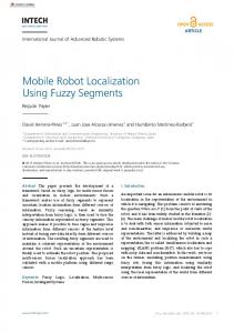
2. The robot platform The experiments were conducted using a Nomad 200 robot equipped with a compass and a ring of 16 Polaroid sonar sensors, as shown in Fig. 1. The sensors are mounted around the robot’s turret, which can be rotated independently relative to the direction of travel. Two other motors located in the base of the robot are used to control the robot’s translational and rotational movements. 2.1. Compass sense A separate behaviour was used to rotate the robot’s turret at small speeds in the direction of ‘North’, as indicated by a flux gate compass, so that the sensors were kept at a constant orientation during self-localisation. The effect of this behaviour was to smooth out local fluctuations in the magnetic field of the robot’s environment.
Fig. 1. The Nomad 200 mobile robot. A flux gate compass was used to keep the turret, and therefore the sensors, at a constant orientation.
120
T. Duckett, U. Nehmzow / Robotics and Autonomous Systems 34 (2001) 117–129
Fig. 2. (a) Raw odometry. (b) Compass-based odometry. The accumulated rotational drift in the robot’s raw odometry was removed on-line using the compass sense.
2.2. Dead-reckoning The compass sense was also used for the on-line dead-reckoning. We used the robot’s wheel encoders to measure the distance travelled, but the rotational component was obtained from the relative angular displacement of the turret against the direction of travel. This had the effect of removing the accumulated rotational drift affecting the robot’s raw odometry (see Fig. 2), because the turret was anchored to ‘North’ by the compass sense, leaving a translational drift error of up to 5% of distance travelled.
which is then used as a stored signature for that place in the topological map (see Fig. 3). In the absence of a compass, we would also have to consider angle histograms, as in [14]. Each occupancy grid cell represents an area of 15 cm × 15 cm, and is considered as being in one of three possible states: occupied (O), empty (E) or unknown (U), depending on the corresponding prob-
3. Representation 3.1. Environment model The robot’s map consists of a set of N stored places, the centre of each place i being associated with a Cartesian coordinate (xi , yi ). Landmark information is also attached to each of the places as follows. Firstly, the robot takes a detailed sonar scan at its current location and a local occupancy grid consisting of 64 × 64 cells is then constructed, as in [28]. However, in our system, we do not store or match the occupancy grids themselves. Instead, each grid is reduced to a pair of histograms (one in x direction, and one in y direction),
Fig. 3. Example occupancy grid and histograms. Occupied cells are shown in black, empty cells in white and unknown cells in grey.
T. Duckett, U. Nehmzow / Robotics and Autonomous Systems 34 (2001) 117–129
121
ability of occupancy for that cell, i.e. O if P (cxy ) > 0.5, State(cxy ) U if P (cxy ) = 0.5, E if P (cxy ) < 0.5,
to produce a pair of histograms. These histograms are then convolved with the corresponding stored histograms for all of the places in the robot’s map. For each stored place i, the matching procedure yields two useful quantities:
where P(cxy ) refers to probability of occupancy for the cell at column x and row y. These probabilities were obtained using the standard method for updating occupancy grids developed by Moravec and Elfes [22]. One histogram is then derived by adding up the total number of occupied, empty and unknown cells in each of the 64 columns, and the other by adding up the totals for each of the 64 rows. Note that the probability P (cxy ) = 0.5 is the default probability used to initialise the cells; this value usually indicates that the cell has not yet been updated because the robot’s view of the corresponding location is occluded by some other object.
1. The strength of the match between the current and stored histograms — this is used to provide a likelihood L(S|hi ) of obtaining the current sensor scan S from each place hypothesis hi . 2. The most likely offset (rxi , ryi ) of the robot in Cartesian space from the centre of the stored grid pattern, i.e. the position in which the sonar scan for that place was originally taken. The first quantity is derived from the product of two separate metrics; one obtained by convolving the current and stored x histograms, and the other by convolving the respective y histograms (Fig. 4). The strength of the match between two histograms T a and T b is calculated using the following evaluation function:
3.2. Location model The robot’s location model consists of a set of competing location hypotheses H = {h1 , . . . , hN }, one for each place i. A probability distribution P = {P (h1 ), P (h2 ), . . . , P (hN )} is associated with set H, reflecting the robot’s belief in each of the hypotheses being its true location. Each location hypothesis consists of a Cartesian coordinate (xhi , yhi ), and a variance vhi which is used for position tracking. Thus, each hypothesis is represented by a simple density function, where the noise around location estimates is assumed to be distributed equally in all directions according to a Gaussian distribution. Obviously, this assumption means that we do not model the robot’s actuators accurately (e.g. by separating the translational and rotational components of robot motion). Nevertheless, we show that the simple mixture model is sufficient for robust navigation performance at low computational cost.
Match(T a , T b ) 1X [min(Oja , Ojb ) + min(Eja , Ejb ) = w j
+min(Uja , Ujb )],
where Oj , Ej and Uj refer to the number of occupied, empty and unknown cells contained in the jth element of histogram T, and w = 64 × 64 is a normalising constant such that 0 6 Match( ) 6 1. In the convolution, the stored histogram is kept stationary and the recognition histogram is translated against it, using the above function to calculate the best match over the 64 elements of the stored histogram. Any non-overlapping elements in the recognition histogram due to the translation are assumed to consist entirely of unknown cells. The likelihood L(S|hi ) is then calculated from the best match scores as L(S|hi ) ∝ Mxi∗ × Myi∗ ,
4. Self-localisation 4.1. Scan matching To begin localisation, the robot takes a new sonar scan. Again, the resulting occupancy grid is processed
(1)
(2)
where Mxi∗ refers to the value of Match( ) produced by the best matching alignment of x histograms for place i. The most likely displacement (rxi , ryi ) of the robot from the centre of each place i is obtained by multiplying the translations for the x and y histograms by
122
T. Duckett, U. Nehmzow / Robotics and Autonomous Systems 34 (2001) 117–129
Fig. 4. Matching the x and y histograms. The new histograms are convolved with the stored histograms for each place in the robot’s map to find the best match.
the dimensions of one grid cell (i.e. 15 cm × 15 cm). The coordinates for each hi are then calculated as xhi = xi + rxi ,
(3)
yhi = yi + ryi ,
(4)
i.e. by combining the coordinates of the place centre and the offset values produced by histogram matching. Finally, to obtain an estimate of the variance in the scan matching, we use the following heuristic function: vhi =
(Mxi∗
k1 k2 + , i 2 i∗ ¯ − Mx ) (My − M¯ yi )2
(5)
where M¯ xi refers to the mean value of Match( ) in the convolution of x histograms for place i, and the constants k1 = k2 = 1.0 m2 in these experiments. 4.2. Multiple hypothesis tracking After carrying out scan matching, the place which yielded the highest match score could be taken as the winner. However, this simple “winner-takes-all” strategy, using only the current sensory input, is bound to fail in complex environments due to factors such as perceptual aliasing and sensor noise. To overcome these problems, we use a succession of sonar scans taken from different positions over time, and apply the following algorithm for accumulating sensory evidence over time.
At each iteration, the algorithm takes as input a prior set of location hypotheses H = {h1 , h2 , . . . , hN } and the corresponding probability distribution P = {P (h1 ), P (h2 ), . . . , P (hN )} from the previous iteration. On initialisation, these sets will be empty. The algorithm can be explained in the following steps. 4.2.1. Initialisation Localisation begins by taking a sonar scan and constructing a set of location hypotheses H = {h1 , . . . , hN }, as described in Section 4.1. For each of these hypotheses, the likelihood L(S|hi ) is obtained using Eq. (2) and the coordinates (xhi , yhi ) are obtained using Eqs. (3) and (4). The initial probability distribution over H is then calculated using L(S|h0j ) P (h0j ) = P 0 . k L(S|hk )
(6)
After initialisation, localisation proceeds as follows. This algorithm is best explained as a three-step predict–match–update cycle (after Crowley [4]). 4.2.2. Predict step Firstly, the robot waits until it has travelled a further 50 cm, then the coordinates (xhi , yhi ) of each of the prior hypotheses hi are translated to take into account the robot motion, using xhi (t) = xhi (t − 1) + 1x,
(7)
yhi (t) = yhi (t − 1) + 1y,
(8)
T. Duckett, U. Nehmzow / Robotics and Autonomous Systems 34 (2001) 117–129
where the vector (1x, 1y) refers to the robot’s own displacement in Cartesian space observed since the previous iteration, using its on-line compass-based odometry (Section 2.2). The additional uncertainty due to the robot motion is approximated by increasing the variance vhi for each of the prior hypotheses as vhi (t) = vhi (t − 1) + k3 ,
(9)
where a value of k3 = 1 m2 was used for these experiments. This constant is based on an approximate estimate of the odometry drift (given that our robot moves a constant distance between scans) plus some extra noise. This has the effect of “blurring” the density function for each of the prior hypotheses. 4.2.3. Match step The robot then takes a new sonar scan, and a second set of candidate hypotheses H0 = {h01 , . . . , h0N }, is created from the new sonar information. In the algorithm presented here, exactly one hypothesis is generated for each place in the map. (Without a compass, we might need to generate several hypotheses per place, corresponding to possible orientations of the robot.) A matching process between the two sets H and H0 then follows. For each new hypothesis h0j , this attempts to find the one most likely equivalent prior hypotheses hi (since only one hypothesis can actually be the “true” location of the robot). Each h0j is therefore compared to every hi , and the likelihood L(h0j |hi ) of obtaining each h0j from each predicted hi is calculated as
123
In the event of a tie, one of the best matching hypotheses is picked randomly. 4.2.4. Update step The likelihood values L(h0j |hj ∗ ) produced by the match step are used to provide a prior probability P (h0j ) by normalising the values produced by Eq. (11). A new probability distribution over H is calculated using Bayes rule as L(S|h0j )P (h0j ) P 0 (h0j ) = P 0 0 . k L(S|hk )P (hk )
(12)
The following equations are then used to update the Cartesian coordinates of each h0j , taking into account the coordinates of both h0j and hj ∗ . xh0j = xhj ∗ + yh0j = yhj ∗ +
vhj ∗ vhj ∗ + vh0j vhj ∗ vhj ∗ + vh0j
(xh0j − xhj ∗ ),
(13)
(yh0j − yhj ∗ ),
(14)
1 1 1 = + . vh0j vhj ∗ vh0j
(15)
The robot then continues to explore, taking a new sonar scan at 50 cm intervals and updating its estimate of its true location by repeating the above process.
5. Experiments 5.1. Experimental procedure
L(h0j |hi ) ∝ G(k(xh0j , yh0j ) − (xhi (t), yhi (t))k)P (hi ),
(10)
where the function G(z) = e−ηz , a monotonic decreasing function of the distance between the means of the two Gaussians, is used to estimate the likelihood of a match, and the constant η = 0.25 in these experiments. The value of G(v) is weighted here by the prior probability P(hi ) in order to take into account the relative weight of evidence afforded to that particular prior hypothesis. For each h0j , the best matching prior hypothesis hj ∗ is therefore defined by 2
∀j : ∀i 6= j ∗ : L(h0j |hj ∗ ) > L(h0j |hi ).
(11)
For the following experiments, robot sensor data were collected in four environments at Manchester University, as summarised in Table 1. The environments were assumed to be unmodified and semi-structured, being subject to transient changes in the robot’s sensor data. People were free to move in the vicinity of the robot, but it was assumed that the basic structural elements such as walls and corridors remained constant with respect to time. The sensor data were recorded by the robot using wall-following, stopping at 50 cm intervals to take sonar scans. Scans were taken by rotating the robot’s turret to obtain three sets of 16 sonar readings at 7.5◦ intervals, yielding a detailed scan consisting of 48 sonar measurements.
124
T. Duckett, U. Nehmzow / Robotics and Autonomous Systems 34 (2001) 117–129
Table 1 Characterisation of environments (the number of places N in the respective maps and the number of trials used for testing in each environment are also shown) Environment
Description
Approximate size
N
Trials
A B C D
T-shaped hallway (some features) Conference room (cluttered) L-shaped corridor (few features) Long straight corridor (very few features)
16 m × 13 m 16 m × 11 m 34 m × 33 m 53 m × 3 m
25 38 69 52
623 478 570 430
In order to evaluate localisation performance, some means of recording the actual location of the robot, referred to as the “ground truth” location, was required. To achieve this, we recorded the robot’s on-line odometry (Fig. 2) during data collection. The collected odometry data were then corrected off-line, by applying a uniform correction factor to the successive laps of each environment to remove the accumulated drift error (see [7] for a full description of this procedure). An example showing the application of this method in a corridor environment is given in Fig. 5. This technique gives us a rough estimate of the robot’s true location. The first lap of the recorded data was then used for map building, and the subsequent laps were used for testing. Given the approximate nature of the ground truth information, we could not measure the exact accuracy of the new self-localisation method. However, the cor-
rected odometer data was sufficiently accurate for us to be able to measure the robot’s performance in global localisation, which is the prime focus of this work. This was achieved by quantising the corrected position data into a set of discrete bins of size 1 m × 1 m. The bin corresponding to the robot’s true location was then taken as the ground truth location. For performance evaluation, the coordinate of the location hypothesis with the highest probability value was taken as the robot’s “predicted” location. To eliminate quantisation errors from the performance measures, a localisation attempt was classified as being correct if the predicted location fell into either the same bin as the ground truth location or into any of the 8 bins adjacent to the ground truth location. In each environment, the proportion of successful localisation attempts was calculated as a percentage of the total number of attempts (“trials”), as given in Table 1.
Fig. 5. Left: environment C in Table 1. Right: retrospectively corrected odometer data used for performance evaluation (see also Fig. 2).
T. Duckett, U. Nehmzow / Robotics and Autonomous Systems 34 (2001) 117–129 Table 2 Scan matching experiment (this shows the percentage of correct localisation attempts for each environment and the mean value µ over all four environments; the mean processor time, T, to match one pair of scans is given in units of t = 1.83×10⁻⁵ s, as measured on a Sparcstation 20) Environment
Occupancy grids
Occupancy histograms
Nearest neighbour
A B C D
57.0% 84.3% 51.4% 33.0%
62.8% 82.0% 55.0% 32.3%
61.2% 73.8% 41.0% 32.0%
µ T
56.4% 13051t
58.0% 31t
52.0% t
5.2. Scan matching First, we assessed the self-localisation performance of the new occupancy histogram matching method without using multiple hypothesis tracking. The performance was compared to that of occupancy grid matching [28], and a third “baseline” method for place recognition, namely a simple nearest neighbour classifier. In the latter system, the vector of 48 sonar readings was normalised, and the dot product was used to determine the best matching place in the map. The self-orientation component of the occupancy grid matching algorithm was disabled here, using our compass sense instead, to enable a fair comparison between the systems. To obtain the map, places were stored at regular intervals of 1 m using the corrected position data taken from the first lap of the ground truth data. Each of the scan matching mechanisms was then tested in each of the four environments using the recorded sonar data from the remaining laps. To assess the computational efficiency of the algorithms, we also measured the mean time taken to match one pair of scans. The results in Table 2 show no measured loss in performance caused by using histograms rather than full occupancy grids, and that this was achieved at a greatly reduced cost in processor time. 5.3. Global localisation Next, we measured the ability of the robot to carry out two tasks using both occupancy histograms and
125
multiple hypothesis tracking: (1) to localise itself under global uncertainty, and then, (2) to recover its position after becoming lost or kidnapped. Again, the experiment was repeated over a large number of trials, as indicated in Table 1, each trial starting from a different (unknown) location along the recorded route data. The performance of the wall-following robot was then measured by playing back the sequence of recorded sonar and uncorrected odometer data starting from that particular location. After travelling a distance of 30 m in each trial, the robot was subjected to a “virtual kidnapping”. This was implemented by transporting the robot back to the beginning of the recorded route data for that particular trial, its odometry being disabled during the move. The results given in Fig. 6 show clearly that the robot is able to localise itself, and remain correctly localised, when starting from an unknown location. Furthermore, the new self-localisation system was able to consistently relocalise the robot after being kidnapped in all of the environments. This was achieved at very low computational cost; for the biggest map of 69 places (environment C), one complete cycle of the new localisation algorithm took 0.003 s on a 600 MHz Pentium III processor. To demonstrate the benefit of using occupancy histogram matching in the new system, we have also shown the performance of multi-hypothesis tracking using the baseline method for scan matching described in Section 5.2. Here, we used the dot product to provide the likelihood L(S|hi ) instead of Eq. (2), and assumed a constant measurement error of vhi = 1.0 m2 instead of using Eq. (5). (This is consistent with our previous algorithm for global localisation with a mixture of Gaussians described in [7].) 5.4. Application to mobile robot navigation Finally, the new self-localisation system has been integrated successfully into a complete navigating mobile robot [6]. This robot has the ability to build its own maps, localise and navigate reliably in unmodified, real world environments containing people which are initially unknown to the robot, without requiring human intervention. Self-localisation is carried out autonomously on-line as part of the navigation process. This was achieved in real-time on the Manchester robot using only its onboard 486
126
T. Duckett, U. Nehmzow / Robotics and Autonomous Systems 34 (2001) 117–129
Fig. 6. Global localisation experiment. This shows the global localisation performance of the new self-localisation system when starting from an unknown location, and then being kidnapped after 30 m of travel. The performance is compared to that of occupancy grid matching, as in Table 2, and global localisation using the baseline method for scan matching described in Section 5.2.
processor, thus demonstrating the efficiency of the new algorithm. In ongoing work, the system has been tested extensively on a second Nomad 200 robot at Örebro University, and has been used to construct a hierarchy of robot maps (see [9] for first results).
6. Conclusions To achieve reliable self-localisation, a mobile robot must depend on its ability to recognise places using landmarks rather than dead-reckoning. Towards this end, Yamauchi and Langley’s approach [28] overcomes some of the problems of using occupancy grids for mobile robot navigation. A globally consis-
tent metric map is not required, because a separate grid is used to represent each place mapped by the robot. Also, the approach does not depend critically on accurate range-finding sensors; similar perceptions produce similar grid patterns, despite the specular effects associated with sonar sensors. However, two major problems remained with this approach until now: (1) occupancy grids require large amounts of storage and computation, and (2) they suffer from perceptual aliasing. We have overcome the first problem by introducing a matching procedure based on occupancy histograms rather than entire grids. To tackle perceptual aliasing, we have developed an efficient algorithm for multiple hypothesis tracking, which does not require the enumeration of a tree of location hypotheses. The uncertainty in the robot’s
T. Duckett, U. Nehmzow / Robotics and Autonomous Systems 34 (2001) 117–129
location model is handled both globally and locally, using a mixture of Gaussian hypotheses to search the space of possible locations. The new self-localisation system has localised successfully in thousands of experimental trials.
7. Discussion In a Kalman filter, the robot’s location model is represented by a unimodal probability distribution which evolves as a Gaussian. By contrast, the new self-localisation algorithm maintains a set of competing Gaussian location hypotheses. The approach can therefore be seen as a multi-modal generalisation on the Kalman filter, because the robot’s location model consists of a mixture of Gaussians, each updated by a separate filter, rather than a single position estimate. However, we note that our approach makes some approximations in its treatment of uncertainty, as discussed in the text, which are modelled more accurately in many Kalman filter implementations (see [12] on optimal linear filtering). So far, we have used a compass to solve the problem of self-orientation. While this method is robust in dealing with minor variations in the magnetic field, severe compass errors caused by ferrous building materials could pose a problem in some environments. A more reliable compass sense could be obtained by integrating perceptual information from the robot’s other sensors, as in the self-orientation system described by Li et al. [21], or by using correlation with a visual map of the ceiling as in [26]. Without a compass, we would also need to consider using angle histograms [14,27]. A related idea can be found in [19], where similar sensor scans were recognised by a clustering algorithm, and a Kalman filter was used to update the robot pose based on the known coordinates of the clusters. Kurz used a technique for pre-processing the scans, known as the most occupied orientation (MOO), which finds the most likely rotational alignment between a pair of scans. However, the MOO strategy would fail in complex environments without a sufficiently accurate prior estimate of the robot’s orientation, due to the problem of rotational aliasing (perceptual aliasing in θ). For global localisation without prior orientation information, we would therefore need to consider multiple hypothesis
127
tracking for the different possible orientations of the robot. The current system contains no mechanism for distinguishing “good” from “bad” sensor data, relying on the robustness of its matching algorithms (due in part to the large overlap between the local grids) to deal with noise and transient variations in the sensor readings. While the system has been tested successfully in several populated environments, such a mechanism might become necessary in highly dynamic environments. One alternative might be to use the entropy-based novelty filter described in [10] to detect any decrease in localisation quality. Such a decrease would indicate some change to the robot’s “expected” view of the environment, in which case the robot could choose to ignore the current sonar readings. The work presented in this paper belongs to a growing family of techniques which integrate map representations at different levels of abstraction and granularity. In many of these, the environment is represented as a patchwork of locally consistent metric spaces connected to form a global topological map (e.g. [9,11,18,24,29]). The new self-localisation system is based on such a scheme. It has been tested successfully as part of a complete navigation system which is able to follow planned paths to user-chosen locations in the robot’s map, where the places are spaced at 1 m intervals [6]. For tasks requiring more precise positioning, the local metric information attached to a particular place could be used for small-scale navigation, as in [11].
References [1] Y. Bar-Shalom, X.-R. Li, Multitarget–Multisensor Tracking: Principles and Techniques, YBS, 1995. [2] J. Borenstein, H.R. Everett, L. Feng, Navigating Mobile Robots: Systems and Techniques, A.K. Peters Ltd., Wellesley, MA, 1996. [3] W. Burgard, A. Derr, D. Fox, A.B. Cremers, Integrating global position estimation and position tracking for mobile robots: The dynamic Markov localization approach, in: Proceedings of the IEEE/RSJ International Conference on Intelligent Robots and Systems (IROS’98), Victoria, BC, 1998. [4] J.L. Crowley, Mathematical foundations of navigation and perception for an autonomous mobile robot, in: Proceedings of the Workshop on Reasoning with Uncertainty in Robotics, Tutorial Paper, 1995.
128
T. Duckett, U. Nehmzow / Robotics and Autonomous Systems 34 (2001) 117–129
[5] F. Dellaert, D. Fox, W. Burgard, S. Thrun, Monte Carlo localization for mobile robots, in: Proceedings of the IEEE International Conference on Robotics and Automation (ICRA ’99), Detroit, MI, 1999. [6] T. Duckett, Concurrent map building and self-localisation for mobile robot navigation, Ph.D. Thesis, Department of Computer Science, University of Manchester, Manchester, UK, 2000. [7] T. Duckett, U. Nehmzow, Mobile robot self-localisation and measurement of performance in middle scale environments, Robotics and Autonomous Systems 24 (1–2) (1998) 57–69. [8] T. Duckett, U. Nehmzow, Performance comparison of landmark recognition systems for navigating mobile robots, in: Proceedings of the 17th National Conference on Artificial Intelligence (AAAI ’2000), Austin, TX, 2000. [9] T. Duckett, A. Saffiotti, Building globally consistent gridmaps from topologies, in: Proceedings of the Sixth International IFAC Symposium on Robot Control (SYROCO), Wien, Austria, 2000. [10] D. Fox, W. Burgard, S. Thrun, Active Markov localisation for mobile robots, Robotics and Autonomous Systems 25 (1998) 195–207. [11] J. Gasós, A. Saffiotti, Integrating fuzzy geometric maps and topological maps for robot navigation, in: Proceedings of the Third International ICSC Symposium on Soft Computing (SOCO ’99), Genova, Italy, 1999, pp. 754–760. [12] A. Gelb, Applied Optimal Estimation, MIT Press, Cambridge, MA, 1974. [13] J. Hertzberg, F. Kirchner, Landmark-based autonomous navigation in sewerage pipes, in: Proceedings of the EUROBOT ’97, Second European Workshop on Advanced Mobile Robots, 1997. [14] R. Hinkel, T. Knieriemen, Environment perception with a laser radar in a fast moving robot, in: Proceedings of the Symposium on Robot Control (SYROCO ’88), Karlsruhe, Germany, 1988. [15] P. Jensfelt, D. Austin, O. Wijk, M. Anderson, Feature based condensation for mobile robot localization, in: Proceedings of the IEEE International Conference on Robotics and Automation (ICRA’2000), San Francisco, CA, 2000. [16] P. Jensfelt, S. Kristensen, Active global localisation for a mobile robot using multiple hypothesis tracking, in: Proceedings of the IEEE International Conference on Robotics and Automation (ICRA’99), Detroit, MI, 1999. [17] S. Koenig, R. Simmons, Xavier: A robot navigation architecture based on partially observable Markov decision process models, in: D. Kortenkamp, R. Bonnasso, R. Murphy (Eds.), Artificial Intelligence Based Mobile Robots: Case Studies of Successful Robot Systems, MIT Press, Cambridge, MA, 1998. [18] B. Kuipers, The spatial semantic hierarcy, Artificial Intelligence 119 (2000) 191–233. [19] A. Kurz, Constructing maps for mobile robot navigation based on ultrasonic range data, IEEE Transactions on Systems Man and Cybernetics — Part B: Cybernetics 26 (2) (1996) 233– 242.
[20] J.J. Leonard, H.F. Durrant-Whyte, Directed Sonar Sensing for Mobile Robot Navigation, Kluwer Academic Publishers, Dordrecht, 1992. [21] G. Li, B. Svensson, A. Lansner, Self-orienting with on-line learning of environmental features, Adaptive Behaviour 6 (3–4) (1998) 535–566. [22] H. Moravec, A. Elfes, High resolution maps from wide angle sonar, in: Proceedings of the IEEE International Conference on Robotics and Automation (ICRA ’85), St. Louis, MO, 1985, IEEE Computer Society Press, pp. 116–121. [23] M. Piasecki, Global localization for mobile robots by multiple hypothesis tracking, Robotics and Autonomous Systems 16 (1995) 93. [24] S. Simhon, G. Dudek, Selecting targets for local reference frames, in: Proceedings of the IEEE International Conference on Robotics and Automation (ICRA’98), Leuven, Belgium, 1998, pp. 2840–2845. [25] S. Thrun, D. Fox, W. Burgard, Monte Carlo localization with mixture proposal distribution, in: Proceedings of the National Conference on Artificial Intelligence (AAAI’2000), Austin, TX, 2000. [26] S. Thrun, M. Benewitz, W. Burgard, A.B. Cremers, F. Dellaert, D. Fox, D. Hähnel, C. Rosenberg, N. Roy, J. Schulte, D. Schulz, MINERVA: A second-generation museum tour-guide robot, in: Proceedings of the IEEE International Conference on Robotics and Automation (ICRA ’99), Detroit, MI, 1999. [27] G. Weiss, E. von Puttkamer, A map based on laser-scans without geometric interpretation, in: Proceedings of Intelligent Autonomous Systems, Vol. 4 (IAS-4), Karlsruhe, Germany, 1995, pp. 403–407. [28] B. Yamauchi, P. Langley, Place recognition in dynamic environments, Journal of Robotic Systems (Mobile Robots, special issue) 14 (2) 1997. [29] U. Zimmer, Embedding local metrical map patches in a globally consistent topological map, in: Proceedings of Underwater Technologies 2000, Tokyo, Japan, May 23–26, 2000.
Tom Ducfrett is currently working as an Assistant Professor in the Centre for Applied Autonomous Sensor Systems at Örebro University in Sweden. In 1991, he graduated from Warwick University with a B.Sc. (Hons.) in Computer and Management Sciences. After working for several years in industry, he returned to academic life and was awarded an M.Sc. with distinction in knowledge based systems by Heriot-Watt University in 1995. His M.Sc. project was carried out at Karlsruhe University in Germany on a system for supporting cooperative computer aided architectural design. He recently completed his Ph.D. Thesis on concurrent map building and self-localisation for mobile robot navigation at Manchester University.
T. Duckett, U. Nehmzow / Robotics and Autonomous Systems 34 (2001) 117–129 Ulrich Nehmzow is a Lecturer in Artificial Intelligence and Robotics at the Department of Computer Science, University of Manchester, leading its Robotics Research Group. He graduated in 1988 from the Technical University of Munich in Electrical Engineering and Information Science (Dipl. Ing.), and obtained a Ph.D. in Artificial Intelligence from the University of Edinburgh in 1992. Following appointments as Research Associate at the Department of Artificial Intelligence, University of Edinburgh, and postdoctoral Research Associate at
129
the Department of Psychology, also at Edinburgh, he became a Lecturer at Manchester in 1994. He is a member of the Institution of Electrical Engineers, member of the IEE Northwest Center Committee, member of the Society for Artificial Intelligence and Simulation of Behaviour, and has worked as Visiting Research Scientist at Carnegie Mellon University and the University of Bremen. In 1999 he was awarded a Royal Society/STA fellowship for a 7-month sabbatical at the Electrotechnical Laboratory in Tsukuba, Japan. His research focusses on autonomous mobile robotics, robot learning, navigation, artificial neural networks, robot simulation and novelty detection.