Research in Electro-optics and Lasers, Orlando FL 32826 USA. IEEE Log Number ..... [7] A. Ghatak, K. Thyagarajan, and M. R. Shenoy, âNumerical analysis of planar optical ... on electronic and crystallographic properties of quasiperiodic ...
JOURNAL OF LIGHTWAVE TECHNOLOGY, VOL. 12, NO. 12, DECEMBER 1994
2066
Modal Fields Calculation Using the Finite Difference Beam Propagation Method Frank Wijnands, Hugo J. W. M. Hoekstra, Gijs J. M. Krijnen, Member, IEEE, and RenC M. de Ridder
Abstract-A method is described to construct modal fields for an arbitrary one- or two-dimensional refractive index structure. An arbitrary starting field is propagated along a complex axis using the slowly varying envelope approximation (SVEA). By choosing suitable values for the step-size, one mode is maximally increased in amplitude on propagating, until convergence has been obtained. For the calculation of the next mode, the mode just found is filtered out, and the procedure starts again. The method is tested for one-dimensionalrefractive index structures, both for nonabsorbing and for absorbing structures, and is shown to give fast convergence.
I. INTRODUCTION
B
EAM Propagation Methods (BPM’s) are very powerful to simulate the propagation of light in structures which cannot be treated analytically. Two frequently used BPM’s are the Fourier Transform BPM (FTBPM) [1]-[3] and the Finite Difference BPM (FDBPM) [4]-[6]. There are various methods to perform a modal analysis for an arbitrary refractive index structure. Two-dimensional transfer matrix methods can be used for two-dimensional structures [7]-[ lo], whereas threedimensional structures require other methods. One method comes down to solving an eigenvalue problem with the dimension of the matrix to be diagonalized being equal to the number of grid points of the cross section [ll]. Another method, by Yevick and I-Iermansson [121, consists of propagating a field distribution along an imaginary propagation direction (throughout this paper, the propagation direction is along the (in general complex) z-axis). The idea is that the guided mode with the highest effective index gets the maximum amplitude increase during propagation. They use as propagation scheme the FTBPM. It is the aim of this paper to show that the FDBPM is quite suitable for solving the modal fields equation. The advantage of the FDBPM is its fast convergence. For the FDBPM the matrix problem can be solved such that selected guided modes can be blown up, as will be shown in this paper. To do so, one may need a large propagation step, which is allowed in the FDBPM. Hence the number of propagation steps in order to blow up a selected mode is in general much smaller for the FDBPM than for the FTBPM. Moreover, the FDBPM gives much more accurate results for large index contrasts (see, e.g., 1131-[151). Manuscript received August 3 1, 1994. F. Wijnands, H. J. W. M. Hoekstra, and R.M. de Ridder are with the MESA Research Institute, University of Twente, 7500 AE Enschede, the Netherlands G. J. M. Krijnen is with the University of Central Florida Center for Research in Electro-optics and Lasers, Orlando FL 32826 USA. IEEE Log Number 9406458.
The waveguide structure to be analyzed is in general zdependent. Since we are interested in finding the modal fields at a cross section of the structure for a given value of z , the given cross section will be extended in the direction of propagation, leading to a z-invariant “calculation structure.” The method is tested for one-dimensional refractive index structures. The method can be easily generalized to twodimensional refractive index structures. The only difference is that the matrix problem is not a tridiagonal matrix problem anymore in that case and hence a different matrix solver should be used than in the one-dimensional case. An efficient iterative matrix solver method is the (preconditioned) conjugate gradient method [ 161. Another, noniterative, matrix solution method is the Alternating Direction Implicit method [ 171, [ 181. A combination of these two methods gives a very efficient algorithm, of which the results will be published elsewhere [19]. The paper is organized as follows. In Section I1 the method is described, both for nonabsorbing and for absorbing structures. Results for some one-dimensional structures are presented in Section 111. A discussion of the results follows in Section IV. 11. THE METHOD A. Propagation Along a Real h i s with FDBPM
In this paper the two-dimensional case is treated. Assuming TE-polarization and a time dependence term eiwt, we have
V 2 E ( z ,z)
+ k,2n2(z,z ) E ( z ,z ) = 0.
A scalar field distribution E ( z ,z) can be written, according to the slowly varying envelope approximation (SVEA), as ~ ( zz ),
(2)
$(z, z)e-ilconoz
where no is a suitably chosen mean refractive index. Substituting (2) into (1) yields
Now $ is assumed to vary slowly as function of z (see (2)). Hence the term d2$/dz2 in (3) can be neglected. Now discretize the field, $j $(sAz,jAz),j = 1,... , N and introduce the vector \E”, ( \ E ” ) j $;. Then (3) is integrated for the discretized field, using the Crank-Nicolson scheme. The result is [5]: AZ 2ikono(\E”+l - \E”) = M(\E”+l+ \E”)-. 2
0733-8724/94$04.00 0 1994 IEEE
1 I1
(1)
1
(4)
..,
WLJNANDS et al.: MODAL FIELDS CALCULATION USING FINITE DIFFERENCE BEAM PROPAGATION METHOD
2067
Here M is a tridiagonal matrix with M i j = &,Mii = &+ki(n:-ni), 1 5 i 5 N , j = i f l , M i j = 0 elsewhere. Transparent boundary conditions are used [20], and efficient interface conditions are applied [14]. For convenience, (4) is rewritten in the form
p+ iMA~/(4kono)]\k"+'= p-
- KO
cc-
KI
iMA~/(4kono)]9".(5)
Here 1is the identity matrix. Following the analysis described in [15], suppose that the propagating field consists of a single guided mode 0"with effective index ne corresponding to the discretized structure. Then 0"satisfies
... Substitution of (6) in (5) yields (7) with say
Pe
ken,, DO
...
...
... I
IAzI [mm]
Fig. 1. Function h;(lAzl),j = 0 , l for two modal fields of bimodal waveguide described in text and AZ purely imaginary. Here no was taken equal to 1.59.
keno. If m guided modes are present, only, then for modal fields with complex effective indexes
each with propagation constant pej,then (7) is replaced by
close to the real axis, the criterion is safe as well. The value for AZ is found from i4,&/Az = T,,S 2 0. Here TO should be estimated, and T,, s 2 1, can be calculated as described below. After having applied (lo), for the next iteration step is replaced by Ts+1
(9) B. Modal Field Solution Using FDBPM
= 7s
fS,f" > +