Model and Procedure for Performance and Availability-wise Parallel Warehouses Pedro Furtado University of Coimbra
[email protected] Abstract. Consider data warehouses as large data repositories queried for analysis and data mining in a variety of application contexts. A query over such data may take a large amount of time to be processed in a regular PC. Consider partitioning the data into a set of PCs (nodes), with either a parallel database server or any database server at each node and an engine-independent middleware. Nodes and network may even not be fully dedicated to the data warehouse. In such a scenario, care must be taken for handling processing heterogeneity and availability, so we study and propose efficient solutions for this. We concentrate on three main contributions: a performance-wise index, measuring relative performance; a replication-degree; a flexible chunkwise organization with on-demand processing. These contributions extend the previous work on de-clustering and replication and are generic in the sense that they can be applied in very different contexts and with different data partitioning approaches. We evaluate their merits with a prototype implementation of the system.
Keywords: de-clustering, replication, parallel processing, load-balancing
1 Introduction Many application contexts find it useful to have a multi-dimensional view of collected data that can be queried, analyzed and mined. These are present in very different environments, such as factories tracking assembly line products, companies tracking and analyzing sales, marketing or financial data, insurance companies tracking insurance-related events and scientific institutions tracking experiments. Accordingly, the corresponding data warehouses may range from a few megabytes to huge giga or terabyte repositories. Those data warehouses must be efficiently queried for pre-planned and ad-hoc analysis. Given that the underlying data sets are frequently extremely large, a panoply of approaches such as materialized views [32] and specialized indexes [33, 34] has been pursued to decrease the processing burden and, above all, to allow the system to return fast results for near-to-interactive data exploration. Strategies based on summarizing the data or indexing it with specialized indexes improve the performance at least for some queries, but only through intensive parallelism is it possible for the system to return fast response times to most queries in very large data sets. Given the huge data and processing burden in large data warehouses, we consider here intra-query parallelism, by cutting either or both the query and data into pieces and assigning those pieces to different processing units. Given several computing units, most data query operations can be processed efficiently in a parallel manner, but then the emphasis
1
concerning large data sets rests on costly I/O and data exchange requirements between computing elements. There are two crucial elements to achieve this kind of parallelism: the parallel architecture and data set partitioning. There is a whole range of architectures for parallelization, from shared-nothing to shared-disk and hybrid ones, and current state-of-the-art servers come with dual- or quad- processors. Each parallel architecture has its own bottlenecks and advantages – e.g a shared-disk architecture shares the storage element among all processing units, as such it places a heavier burden on I/O and interconnects from the shared storage to computing elements, which may limit scalability and must be compensated by specialized hardware and software features. Shared-nothing architectures are a simple and effective way to benefit from the storage and processing elements of off-the-shelf PCs, and a scalable solution can be put together with 10, 20 or 100 low-cost PCs (given that current COTS PCs are themselves dual or quad-processors, the solution is itself a hybrid parallel architecture). In such an architecture, each node has its own data (partition) and either on-the-fly (on a need base) or placement-dictated replication is very useful if efficient load and availability balancing are to be achieved. Given that on-the-fly data transfers are time consuming, not only due to the data transfer over the network, but also due to the node burden sending and receiving the dataset, the system should try to place and replicate the data as well as possible to allow the maximum degree of load-balancing without on-the-fly data transfers. Partitioning [27] is a pre-condition for parallel processing, but its application scope is larger than that. It refers to splitting huge data sets, such as data warehouse fact tables, into much smaller pieces that can be handled efficiently. For instance, if the data is partitioned on an yearly basis, a query requesting only the sales of the last year needs only process a partition that corresponds to last years’ data. Partitioning can be horizontal – table rows - or vertical – table columns. Both approaches have been used before, although horizontal partitioning is the most widely used approach in commercial systems. Most commercial database systems currently offer native support for horizontal partitioning based on ranges, lists or has-values, and include SQL-DDL constructs and implementation of those partitioning approaches. Another difference is that vertical partitioning involves some degree of redundancy, as the attribute(s) to be included in fragments are accompanied by some common key attribute that identifies the corresponding table row. Since horizontal partitioning is the most widely supported approach, without the kind of redundancy of vertical approaches and renders itself well to parallelization, we concentrate on that alternative throughout this paper. Horizontal-partitioning may be “Attribute-wise” - a partitioning that is determined by the values of one or a combination of attributes. For instance, if sales data is partitioned by shop and product and a query requests a specific shop and product, only a partition needs to be processed to answer the query. Partitioning is also a pre-condition for efficient parallel processing by any architecture: if there is more than a single processing unit, parts of the data must be allocated to each processing unit, and those parts are the partitions. There have been several proposals in the past concerning data warehouse partitioning and parallel processing that can be used in a shared-nothing context, of which we mention a few:
2
MDHF [24] used workload-based attribute-wise derived partitioning of facts and in-memory retention of dimensions for efficient processing. It introduced the use of join-bitmap indexes together with attribute-wise derived partitioning and hierarchy-aware processing for very efficient partition-wise processing over star schemas; The Data Warehouse Stripping system [4] used round-robin partitioning of facts and copy of dimensions; The Data Warehouse Parallel Architecture [7, 8, 9, 10] uses hash-based partitioning of large relations and copies of smaller ones; The approach in [2] proposes a genetic algorithm for schema partitioning selection, whereby the fact table is fragmented based on the partitioning schemas of dimension tables. Partition-handling, load-balancing and availability-related flexibility are crucial for efficient operation over possibly heterogeneous nodes and network segments. Network segments may go offline, nodes may process at very different speeds and, depending on the application context, some nodes and network segments may even not be dedicated exclusively to the warehouse operation. What is necessary is a flexible, data warehouse-related, partition-handling approach for load and availability-balancing. We also want the approaches to be generic, in the sense that they define principles that can be applied regardless of underlying choices such as partitioning approach details. We define chunks as partitions with specialized load and availability balancing concerns and characteristics. Our emphasis is to limit the amount of replication needed for top performance in this environment, to develop a model to assess the value of placement and replication alternatives, and to determine how to handle heterogeneity and non-dedication over the placement to deliver top efficiency and availability. With a careful approach to chunk-based de-clustering and replication, we can for instance reduce the total mirroring storage from 100GB x 10 nodes = 1TB to a partial replication storage of 300GB, avoid huge loading times and still have a very efficient system. Given these objectives, our important contributions to current knowledge are: 1. We propose a simple and very effective chunk-wise approach with on-demand processing for load and availability balancing over the parallel data warehouse; 2. We introduce and apply a performanceindex that is crucial for effective load-balancing; 3. We give a formulation for the performanceindex based placement and for the replication-degree issue (decision on how much to replicate); 4. We introduce both a model and a predictor for the approaches; 5. We use these together and show experimentally that the solution effectively balances the system and the predictor is useful. To the best of our knowledge, these contributions innovate in several respects that include the formulation and algorithms for optimized allocation with the performance-index measures; upper and lower bounds on prediction of performance as a function of the performance indexes; the algorithmic basis for the predictor of the effect on performance of different allocation and replication schemes; load-balancing friendly performance-index wise allocation algorithms; applying dynamic loadbalancing with in this context, evaluating experimentally the effect in performance with varying number of replicas and assumed performance index and plugging the experimental data on the predictor to show that it can be used to assess a placement-replication scheme.
3
Section 2 reviews related work. In section 3 we present the model for chunk-based performance-wise placement and replication. Section 4 discusses chunk-wise on-demand processing for load and availability balancing. In section 5 we evaluate the approaches and section 6 concludes the paper.
2 Related Work In the past, there has been a lot of work on implementing data management systems over conventional shared-nothing architectures, as reviewed in [5]. Partitioning, processing, replication and load-balancing are all relevant issues concerning intra-task parallelism in shared-nothing architectures with large data sets and heterogeneity-handling. We will first review basic partitioning in parallel databases and data warehouses in section 2.1, and then in section 2.2 we focus on OLAP processing, replication and load-balancing, which are central to our proposals.
2.1. Data Partitioning Partitioning is a pre-requisite for parallel processing over the data warehouse. For this reason we review data partitioning in this subsection. Our models for chunk-based, performance-wise load and availability balancing are generic, in the sense that they can be applied to different partitioning solutions discussed next. In relational databases there are two major partitioning perspectives to be considered (one can also consider mixes among them) [27]: horizontal and vertical partitioning. Horizontal partitioning refers to partitioning relations by rows, that is, each row will belong to one of the partitions. Vertical partitioning, on the other hand, refers to creating partitions consisting of one or more columns of a relation. Naturally, researchers have looked for efficient partitioning and placement alternatives in the case of a database processing generic workloads. Williams and Zhou [28] review five major data placement strategies (size-based, access frequency-based and network traffic based) and conclude experimentally that the way data is placed in a shared-nothing environment can have considerable effect on performance. Hua and Lee [15] use variable partitioning (size and access frequencybased) and conclude that partitioning increases throughput for short transactions but complex transactions involving several large joins result in reduced throughput with increased partitioning. These works consider generic workloads, while our effort concerns intra-task optimized parallelism. Horizontal partitioning is the most widely used approach and most database engines provide SQL primitives for automatically partitioning the datasets, with the choice of partitioning key or keys and partitioning criteria. Typical criteria are range, list, hash and composite. For the first two, the user provides a range or a list of key values and the system automatically places the data into the correct partition based on the key value. Hash partitioning involves hashing the key value according to a function, such that the partition is determined based on the hash result, and composite criteria are mixes of the previous ones. Partitioning can also be done irrespective of the
4
key values. This is the case with round-robin partitioning in which rows are assigned different partitions in a round-robin fashion. Hash and round-robin were pointed-out as two practical partitioning solutions for parallel databases [5] and examples of parallel data warehouse prototypes using them include DWS [4], which uses round-robin partitioning of facts and copy of dimensions, and DWPA [7, 8, 9], which uses hash-based partitioning of large relations and copies of smaller ones. There are important reasons for hash-partitioning relations related to minimizing data exchange requirements in parallel join processing [16]. Parallel hash-join algorithms are also reviewed in [29] and by equihashing relations that are to be joined the processor saves a lot of overhead associated with the necessity of exchanging data between nodes in order to send tuples into the node that has been allocated the corresponding hash-value range for the join attribute. Several works have focused on deciding the best hash layouts workload-wise so as to maximize the equi-hash opportunities and these ways minimize join-related data exchange overheads among shared-nothing nodes [23, 29]. We denote as attribute-wise derived partitioning as the partitioning of a relation using attributes from one or more other relations. This kind of partitioning is possible if the relations have join attributes among them and it is very useful for the star schemas of parallel data warehouses, since it optimizes joins. Attribute-wise derived partitioning proved to be very efficient in both [24] and [2], as it allows the query processor to access only the necessary partitions. In particular, the work in [24] further introduced the use of join-bitmap indexes together with attribute-wise derived partitioning and hierarchy-aware processing for very efficient partition-wise processing over star schemas. Given a basic partitioning approach, replication and load-balancing become the essential tools to optimize processing efficiency in the presence of heterogeneity, skews and faults. We discuss work on these issues in the next subsection.
2.2. Replication, Processing and Load-Balancing The use of replication for availability and load-balancing has been a subject of research for quite a while now. There are multiple levels at which to consider the replication issue. Mirrored disk drives [26] and RAID disks [22] are examples of storage organization level proposals; Multiple RAID alternatives were proposed, some emphasizing only reliability advantages, others with performance and reliability on their sight. At the networked data level, the concept of distributed RAID (ds-RAID) [25] glues together distributed storage by software or middleware in a network-based cluster. The Petal project [17] built a prototype of ds-RAID and the work in [11] further evolved the concept with an orthogonal striping and mirroring approach. These approaches are low-level data-block ones similar to RAID approaches, but at the networked multiple-nodes level. Their basic concepts are useful for parallel data warehousing, but they must be applied at a higher partition and processing units-level, since disk block-wise solutions would not spare very expensive data transfers from the disks to the processing PCs to retrieve whole partitions if we were to use them in our setup.
5
At the OLAP query-processing level, the most closely related works to this one are [1, 3, 20, 21]. In [1] the authors propose efficient data processing in a database cluster by means of full mirroring and creating multiple node-bound sub-queries for a query by adding predicates. This way, each node receives a sub-query and is forced to execute over a subset of the data, called a virtual partition. Virtual partitions are more flexible than physical ones, since only the ranges need to be changed. The authors of [20] further improve the previous solution. They claim that the solution is slow because it does not prevent full table scans when the range is not small, and propose multiple small sub-queries by node instead of just one [21], and an adaptive partition size tuning approach [20]. The rationale in both [1] and [20, 21] still suffer from data accessperformance related limitations: full table scanning as in [1] by every or most nodes is more expensive than having each node access only a part of the data; the alternative in [20, 21] of reducing the query predicate sizes to avoid full table scans also has another limitation in that it assumes some form of index-based access instead of full scans. Unless the data is clustered indexkey-wise (which should not be assumed), this can be slow for queries that need to go through large fractions of data sets (frequent in OLAP). These limitations are absent in partitioned data sets, as long as the query processor is able to restrict which partitions to access. Chunks are just fixed size partitions, with the added restriction that their size must be such that they can be used for replication and efficient load-balancing. Our basic partitioning into chunks can be implemented in any relational database management system (RDBMS), by either creating separate tables for each chunk or using the partitioning interface offered by it. In the case of IBM DB2 server [30], it allows the definition of any number of partitions (up to some limit) for dividing tables into a set of nodes, and small tables can be copied across all nodes. In that system parallel joins are processed in different manners, depending on the co-location status of joining relations: In co-located joins the data is already partitioned according to the join hash values, so the join can occur in parallel with no data exchange requirements between nodes; In redirected joins the data is not co-located but it is enough to relocate the rows from one of the source data sets in order to co-locate them and proceed with a colocated join; In repartitioned join: both source data sets need to be re-located in order to become co-located; In broadcast join one of the source data is broadcasted into all nodes to enable parallel joining with the other partitioned data set; Chained de-clustering [12, 13, 14] is also a relevant related work, as the proposed solutions avoid full mirroring and provide availability. Our models are inspired in chained-declustering, but the original chained-declustering proposal is targeted at individual relations and do not use chunking but rather node-wise partitions, whereas we define our approach regarding a data warehouse schema, where small dimensions are copied instead of partitioned. The absence of chunks makes chained declustering less convenient for dynamic load-balancing, due to static chain processing assignment: in chained-declustering, each node has a partition and the whole image of that node is entirely copied into one immediate neighbor; to replace parts of the processing of a node under this placement, we need a rippling effect - each node has to process a predefined fraction of the previous node’s data and a predefined fraction of its own data. This is too static for dynamic load-balancing and also suffers from an index-related access requirement for processing
6
only parts of partitions. Our design solves these issues by placing and accessing replica chunks instead of full image backups, so that we never have to process only parts of a partition (the index issue), we can use chunks as replication units and we can assign chunk processing very flexibly through on-demand load-balancing. Our previous work on this subject included [3], which used full mirroring for availability and performance, and [6], which proposes chunk-wise placement for availability only, without loadbalancing considerations or on-demand processing. We extend these two works by considering partial replication instead of full replication, and dynamic load and availability balancing for very efficient and available node-partitioned data warehouses. In what concerns load-balancing specifically, there is a very large body of related work and we refer the reader to the review in [18] and the thesis [19], where the author compares a wide range of approaches and concludes for on-demand, task stealing load-balancing. On-demand loadbalancing, where consumers ask for further tasks as soon as they end the last one given to them, allows the system to adapt automatically and dynamically to different and varying skew, heterogeneity and non-dedication conditions. In the next section we present the performance-wise model, which is the basis for our chunkbased efficient solution.
3. Performance-Wise Model Performance-wise chunking is a simple concept, but in order to explain it, we must define chunk and chunk replication as well. In this work, we define chunk as a partition of a dataset with a predefined target size. The concept of chunk is stricter than the concept of partition, in the sense that it defines a target size for the partitions. Just as a disk has data blocks, and those blocks can be copied (replicated) into other disks to alleviate hot spots, higher-level chunks will have equivalent functionality. While partitions or fragments focus on query processing optimization, chunks also target load and availability balancing, so that size and replication are the central issues for them. A chunk replica is a copy of a chunk, which resides in a different node from the original chunk. Given chunks, performance-wise chunk placement and replication is the process of determining how the chunks can best be placed to deliver the best possible efficiency without full-mirroring (that is, without copying every chunk into every node). In the next sections we discuss chunk determination and processing. Then we derive the model for performance-wise placement and replication of chunks.
3.1. Warehouse Schemas, Chunk Determination and Processing In this section we first discuss warehouse schema partitioning and then review briefly information on basic assumptions on chunk characteristics and processing that are used throughout the rest of the work. In relational databases, Data Warehouses are frequently organized as star schemas [31], with a huge fact table that is related to several dimension tables, as represented in Figure 1. In such
7
schema, the facts table (Sales fact in the Figure) stores data to be analyzed and pointers to dimensions, while dimension information is stored in dimension tables (the remaining relations).
Figure 1. DW Sample Star Schema It is frequent for dimension tables to be orders of magnitude smaller than the fact table. When considering a parallel environment, this means that it is worth to partition the central fact table into multiple pieces that can be processed in parallel, while the dimension tables are left complete. In a shared-nothing environment, this means copying dimension relations into all nodes and dividing the fact throughout the nodes. This approach is very useful in what concerns parallel processing, since most operations can proceed in parallel [10], including processing of joins in parallel. In this work we assume this organization of the schema within a parallel architecture, or an extension whereby there may be more than one partitioned relation as long as they are co-located [7, 8, 9]. In our experiments with the TPC-H benchmark we did this: Lineitem relation was hash-partitioned (partitioned based on hash-ranges) and relation Orders was co-located with Lineitem (the same hash-ranges were used), while the remaining smaller dimension relations were all copied into all nodes. Some more complex schemas may include bigger dimensions and multiple interconnected big relations that, for best performance, need to be partitioned, and it may happen that it is impossible to partition all for co-location. We discuss and provide solutions for this in [7, 8, 9]. In those cases, when two datasets that need to be joined are both partitioned and not co-located, there is a need to re-partition at least one of the datasets on-the-fly to do the join. We will extend our current proposals to optimize this kind of case in future work. The first issue concerning chunks is to define and enforce a convenient size, since chunks are the individual units that can be placed and processed in a highly flexible fashion, regardless of the partitioning approach. Since the focus of this work is on replication degree, load and availability balancing, and the solutions proposed are to be used generically with different partitioning approaches, we assume chunk target size and target size enforcement to be guaranteed by the partitioning approach itself and refer to these issues only briefly. We assume a target chunk size value (e.g. in our experiments with TPC-H our target was approximately 450MB for base Lineitem table, which we then rounded up to get exactly 30
8
chunks), noting that there is a fairly wide range of acceptable chunk size values which yield good performance, given a simple guiding principle: if there are too many very small chunks, there will be a large extra overhead related to switching disk scans among chunks, collecting partial results from each and merging all the results; If, on the other hand, the chunk is too large, we will not take full advantage of load-balancing opportunities. Chunk target size enforcement is dependent on the partitioning approach. A chunk target size is a simple and always available way to influence the number and size of pieces that are an input to the allocation approach, which in turn is useful for the dynamic chunk-wise load and availabilitybalance. In contrast with what would be more sophisticated alternatives for optimization of chunk configuration, such as a benchmark or workload-based analysis, the simple specification of a chunk target size does not require further knowledge and adds only a simple target-related soft constraint to a partitioning approach. The target size objective can then be applied with any partitioning criteria – whether hash-based, round-robin, random, range-based or derived (dimension-attribute wise). For instance, given a dataset with size S and a target chunk size of C, the number of hash-buckets n in hash-based partitioning should be n=S/C, therefore chunk size enforcement is based on defining and reorganizing hash-range sizes (and chunks) accordingly when the actual chunk sizes rise above an upper limit beyond the chunk target size; In Roundrobin or Random partitioning, the number of chunks is n=S/C and the rows are divided in roundrobin or random fashion over those chunks; In dimension-attribute wise partitioning criteria, the target is used as an additional element in the determination of the attributes to use in the partitioning decision, as these are influenced by both workload-based determination of a suitable set of attributes and the desired number or size of chunks, as in [24]. Since there may be skew in the resulting chunks, skew-resistant partitioning approaches for hash, range and attribute-wise partitioning is a relevant related research issue for future work. Apart from the load and availability issues which we will consider in subsequent sections, chunk-wise query processing considerations are not different from basic query processing over partitions [1, 10, 7], of which we review the common aggregation operation here. Data warehouses are usually target of queries with aggregate operators, like sum, count and average. Figure 2 presents an example of query transformations for the sum operator over a fragmented table (sales), where Nc is the number of chunks that make up a partitioned dataset. (a)
Initial query
Select regionID, sum(sales) From JOINpkey sales, product Where Group by regionID;
(b)
Rewritten query for chunk i
R(i):= Select regionID, sum(sales) From JOINpkey salesChunk_i, product Where Group by regionID;
(c)
Generating the final result
U= Union(R(i)), i=1 to Nc Result:=select regionID, sum(sales) From U Group by regionID;
Figure 2. Query transformations for Processing Chunks/Partitions in Parallel The initial query over a Sales fact (Figure 2-a) is transformed into several others ones, each one over a chunk of the table (Figure 2-b). The transformed queries (Figure 2-b) access individual chunks of the table. After the rewritten queries are executed, their results must be merged in order to generate the final result of the originally submitted query. In Figure 2-c, we present an example of the merging step for the sum operator. After the rewritten queries are executed, their results are combined by a union relational operation (forming the relation U, in the example). A simple select
9
over the U relation gives the result of the original query. Depending on the operators used at the original query, distinct transformations and merge operations must be done. In [10] the author presents several examples on query transformations and results merging operations. Chunk-wise processing generates a result R(i) per chunk, which must be merged to obtain the final result (Figure 2-c). We will see in the on-demand load-balancing algorithm that, as soon as a node ends processing chunks, it starts merging its local results and then sending the result to a merger node, and when all nodes end processing all the chunks, a merger node applies the final merge query. This simple example also serves as an illustration to why the target chunk size should be determined in a workload-based manner, as we pointed out above: the most appropriate chunk should be one that does not result in excessive extra overheads, which is related in Figure 2 to the number and size of the partial results R(i) per chunk, and the size of R(i) in this case depends on the cardinality of the regionsID attribute. In this paper we focus chunk processing for queries such as the one shown in Figure 2. In future work we intend to generalize these approaches to handle more complex schemas and query processing cases for which the basic query processing in shared-nothing architectures was described in [10]. The solutions and models described in this work can be applied in different contexts, from specialized parallel database servers to engine-independent parallel processing middleware over any database engine. This is because there is no need for specialized modifications to a database engine to handle chunks, as only a chunk-wise processing middleware is required, while chunks can be stored as relation partitions or as relations themselves. Our prototype implementation uses the Data Warehouse Parallel Architecture [7], developed as a generic middleware over any database engine to achieve engine-independence. The prototype uses regular tables to store chunks, and the experiments were ran over postgres-SQL databases.
3.2. Placement, Replication and Load Balancing In this section we briefly introduce and review the base placement and replication concepts over which we will discuss performance indexes and advanced solutions in the subsequent sections. Homogeneous placement refers to the basic chunk placement approach, under which the data is placed into the nodes of the parallel data warehouse so that all disks have approximately the same amount of data. Replication is crucially applied in shared-nothing environments for availability reasons, so that if a node fails the other nodes replace its processing [12]. It is also useful for loadbalancing in the presence of heterogeneity. Load-balancing is achieved by faster nodes replacing slower ones in the processing of chunks, on-demand meaning that a node asks for further work as soon as it ends processing. We consider that transferring the necessary chunks from a node to another one on-the-fly (during the processing of a query) is costly (the overhead of reading from disk or memory and transferring all relevant chunks from a node, plus the cost of receiving and storing in disk or memory in the other node), so that on-demand load-balancing relies on chunk replicas that are already in the node. Optimal load-balanced processing is obtained by replicating all chunks into all nodes (mirroring), as a faster node can always help slower ones by finding
10
chunks that need processing in their replica set. However, mirroring data sets adds significant update/load costs besides unnecessary storage costs. It is much more tempting to find the number and placement algorithm for replicas such that processing runs sufficiently fast without the need for full replication. The amount of replication that is required –degree of replication –depends on the heterogeneity of the nodes, data skew and dynamic heterogeneity factors such as variations in processing due to external loads. In theory, a system that is homogeneous in all these factors (same node characteristics, no data skew and no dynamic changes) would need no replicas - execution is balanced, while a very heterogeneous (or non-dedicated) environment requires many replicas and an improved placement to handle unbalance. In the next section we discuss this issue and provide solutions. From this point on we use the terms full mirroring and full replication interchangeably.
3.3. Performance Indexes and Model Consider a set of Nn PCs, processing a total of Nc chunks at homogeneous speeds, and assume that the average time over all nodes to process a chunk is tc (the average time to process a chunk by node i is denoted as tc(i)). With homogeneous placement and no replication, the time cost of processing all chunks is, (1) Since in this case PCs are homogeneous, this cost is the same with or without full mirroring. Now assume a system where PCs process at different speeds (due to heterogeneity and/or nondedication) and call “Performance Index” (PI) the speed comparison factor: Definition 1 (Performance Index PI): The performance index is a number specifying how much faster a PC processes a chunk than the slowest PC in the system. This value should be statistically collected, based on the performance of the nodes processing similar chunks. Consider this definition and an average time to process a chunk by node i given by tc(i). The average time to process a chunk by the slowest node is tc(clowest).Then, the slowest PC has PI=1 and the remaining PCs have, ,
(2)
Higher performance indexes mean faster. The performance index is a generic measure of heterogeneity in processing chunks. We can measure it offline or use the values obtained during the processing of the queries; we can have a measurement over a long time span or use the latest measured value to account for current “noise” in the form of non-dedicated nodes doing some other stuff besides processing the data warehouse queries. We propose an allocation-time procedure for computation of the performance indexes: 1.
Input to the approach: workload: queries with frequency, schema;
2.
Allocate all dimensions to all nodes;
3.
Allocate at least a fraction of the chunks (e.g. 50%) to all nodes homogeneously;
4.
Run the queries over all nodes according to the query frequencies, obtaining an average chunk processing time statistic tc(i) in each node i;
11
5.
Collect all tc(i) values, the largest values is t(slowest).
6.
Compute PI(i) = tc(i)/t(slowest), for all nodes.
After the performance indexes are computed as explained above, allocation and processing can begin using them. The above-described procedure is an allocation-time computation. The performance indexes can also be updated as nodes participate in queries along time. For instance, update their values every n queries (n being a configurable parameter) with the average per-chunk processing times tc(i) for those queries. Consider in a generic case that node N(i) processes Nc(i) chunks and the average time it takes to process a chunk is tc(i). Given any placement, replication and processing approaches, one important thing is to determine how close the approach is to an “optimal” processing time.
We
give the following definitions and expression for optimal processing time and for the worst processing time: Definition 2 (Optimal Processing Time): The optimal processing time is the least time that the system can take to process a query considering all nodes have all the data available (full mirroring). Lemma 1 (Optimal Processing Time): Equation (2) gives the optimal processing time: (3)
Proof: as every node has all the data, we will consider on-demand processing, where each node requests a new chunk when it ended the previous one. We also assume that all nodes end at the same time, which is true if chunks are infinitesimally small under on-demand (and it is also an acceptable assumption in practice if chunks are not very large). All nodes take the same total time, denoted as Tc(i) for node i: (4)
The sum of all chunks processed by all nodes is the number of chunks processed Nc. Using that expression and (4) and considering some node j,
(5)
Solving this expression for N(j), (6)
So, (6) states that any node j processes
of the chunks in the data set. Given that
the time taken to process is equal for all nodes in the optimal case, we can consider the slowest node. Since in that case PI(slowest)=1 (by definition of PI), then the slowest node
12
processes
chunks. Given that the average time to process a chunk is tc(slowest) for
that node, we reach expression (3), as desired.
Definition 3 (Worst Processing Time): The worst processing time is the time taken by the system assuming homogeneous placement with no chunk replication. This time is given by equation (7), (7) Proof: Since the worst processing time corresponds to homogeneous placement, each node has
chunks, and the system ends processing when the slowest node ends. Since the slowest
node takes time tc(slowest) per chunk, it takes (7) to process all chunks. Example 1: consider a parallel warehouse with 5 nodes, PI values (1,2,4,5,7) and a slowest node taking an average of 30 secs to process a chunk. If the dataset has 80 chunks, the optimal time to process this dataset is . The worst processing time, which corresponds to the time taken to process the query with homogeneous placement and no replication, is . This example shows that we can predict the optimal and the worst time for any node configurations. Given that we wish to minimize the need for replication, what we want is to have partial replication and/or non-homogeneous placement schemes instead of full mirroring into all nodes, returning times close to full replication without requiring full replication itself. Definition 4 (Processing Time with r Replicas): The processing time with r replicas is the time taken by the system assuming every chunk has r replicas. Consider a relation R with size S(R). Since each chunk has r replicas, this also means that R will have a total size of with replicas. The time taken with r replicas depends on a few factors, including placement of chunks and chunk replicas. We have built a simple computerized model that simulates chunk and chunk replica placement following simple policies, which we discuss in the next section. The model then runs an event-based simulation of the processing, following the algorithms that we define in subsequent sections, and outputs expected times. The simulation itself uses as parameters the variables Nn, Nc, PI(i), tc(slowest) and r given above and returns the expected time to process the data. Using tc(slowest) and the performance indexes to compute chunk processing times, the simulation jumps from event to event, where events are chunk processing completion times, and this way predicts the time to process the whole dataset very fast. With this model we compute expected chunk-wise processing times, as in the next example. Example 2: In the previous example, and considering homogeneous placement (every node has the same amount of chunks) and the offsetting of replicas to neighbor nodes, the times taken to process the 80 chunks with r replicas each in 5 nodes and PI indexes PI(i) = {1,2,4,5,7} are given in Figure 3. The Figure shows: the optimal time (opt), as given by equation (3); the worst time (worst), as given by equation (7); and the actual time taken in the model with 1, 2 or 3 replicas, as
13
given by the curve named “homogeneous”. From this example we can see that the worst time coincides with the no-replica homogeneous results. We can also see that with a replica (r=1) the time taken is reduced from 480 to 180 secs and more replicas achieve a runtime near the optimal. In practice, they achieve a runtime of 150 secs versus 126 secs for the optimal. Recall that, in the proof of lemma 1 concerning the optimal time, we assumed that all nodes end at the same time. This is why the simulated time to process all chunks is not exactly the same as the optimal, as in practice one or more nodes are idle while other nodes process their last chunk. (note: the difference between the optimal and the actual time taken could be decreased a bit further using work-stealing algorithms [18, 19], under which faster nodes that end processing can steal currently running chunks to end their processing faster).
Figure 3. Time versus Number of Replicas
3.4. Basic Chunk Replica Placement While replicating chunks, we must make sure that a replica does not end in the same node that has the original chunk and we must make sure that the various chunks of a node are replicated into different nodes, so that load and availability-balancing is effective. Inspired by the approach of chained de-clustering, which would copy entire node images to a neighbor node, we chain the chunks of a node into consecutive nodes in round-robin fashion, as shown in the algorithm of Figure 4. In lines 2. to 4. the chunk replicas from node i are placed consecutively in the other nodes and in lines 5. and 6. we avoid placing a chunk replica in the chunk primary node. This approach achieves a completely balanced placement for replicas. Algorithm 1. (Placing number_of_replicas replicas for node i): 0. FOR r=0 to number_of_replicas-1 1. currentNodeForChunk=i+1+r MOD Nn; 2. FOR j=1 to number of chunks Nc(i) of node N(i) 3. add chunk j to node N(currentNodeForchunk) MOD Nn 4. currentNodeForChunk+=1; 5. if(currentNodeForChunk==i) 6. currentNodeForChunk+=1;
Figure 4.Replica chunk chain algorithm
3.6. Performance-wise Placement and Replication Given the Performance-index, it makes sense to place or replicate the chunks in a performancewise manner, which means that each node will have an amount of chunks (original or replica) that is proportional to its relative performance in the system.
14
Performance-Index based placement tries to place chunks according to performance-indexes in the first place. Since the optimality objective is to have nodes processing
chunks, and
if there were no variations in processing time, we would need no replication at all if we would place chunks in a performance-wise fashion, so that each node would have exactly that number of chunks. In practice, the performance index is a statistical value and the actual relative performance may vary both temporarily and permanently with factors such as the queries, evolution of the data in the nodes and many external factors such as non-dedication of the nodes. Still, placing the chunks according to statistical performance evidence, together with some degree of replication and load balancing is important. We give next the performance-wise placement algorithm (with either round-robin or random assignment). The algorithm verifies in step (1.) in which interval of the cumulative distribution of performance indexes a random number (or the chunk ID in round-robin) generated within that interval will fall, assigning the chunk to the node that corresponds to that interval. Algorithm 2 (Performance-wise Placement): Consider the nodes numbered from 0 to Nn-1 and a simple structure with Nn positions, with the cumulative values of performance indexes defined as follows: (8) The algorithm is, for i in 1 to Nc Round-Robin: 0. place chunk(i) at N(j) such that 1. cumPI(j-1) < i MOD cumPI(Nn-1) Seq Scan on lineitem (cost=0.00..2566076.80 rows=58270496) (actual time=13.936..226621.916 rows=59142609 loops=1)" " Filter: (l_shipdate = date '1994-01-01' and o_orderdate < date '1994-01-01' + interval '1 year' group by n_name order by n_name;
25
Appendix B – Explain Plan for Queries Q1 and Q12 from TPC-H
Appendix B shows the costs and runtimes or the standalone run (run of the query on a single node) and both the cost and runtime of processing a chunk query. We obtained these execution plans during the setup of the experimentas to assess the advantage of parallel, node-partitioned chunk processing. Q1 Standalone (Fast Nodes):
Q1 Chunk:
"Sort (cost=4022839.55..4022839.56 rows=6 width=51)
"Sort (cost=134038.02..134038.04 rows=6 width=51)"
(actual time=1504601.262..1504601.265 rows=4 loops=1)"
" Sort Key: l_returnflag, l_linestatus"
" Sort Key: l_returnflag, l_linestatus"
" -> HashAggregate (cost=134037.67..134037.95 rows=6)
"->HashAggregate (cost=4022839.20..4022839.47 rows=6 width=51)
"
"
-> Seq Scan on lineitemorderkey13
-> Seq Scan on lineitem (cost=0.00..2566076.80 rows=58270496)
(cost=0.00..85538.38 rows=1939972 width=51)"
(actual time=13.936..226621.916 rows=59142609 loops=1)" "
Filter: (l_shipdate