Model Approximation for HEXQ Hierarchical Reinforcement Learning Bernhard Hengst National ICT Australia, University of New South Wales, Sydney NSW 2052, Australia
[email protected]
Abstract. HEXQ is a reinforcement learning algorithm that discovers hierarchical structure automatically. The generated task hierarchy represents the problem at different levels of abstraction. In this paper we extend HEXQ with heuristics that automatically approximate the structure of the task hierarchy. Construction, learning and execution time, as well as storage requirements of a task hierarchy may be significantly reduced and traded off against solution quality.
1
Introduction
Not only do humans have the ability to form abstractions, but we control the amount of detail required to represent complex situations for decision making. Take the familiar problem of deciding the best way to travel to a business conference or holiday destination. We first choose the mode of transport and best route between major cities. To make this decision we may even take into consideration potential connections and delays at either end for each mode of primary transport. However, the side we get out of bed on the morning of departure or the way we leave our home (front door, back door or garage door) is unlikely to be an influencing factor in our decision, although in the final execution of the plan will need to decide to get out of the bed on one side and use one of the doors to exit the home. How can a reinforcement learner model these pragmatics? Interestingly, hierarchical reinforcement learning (HRL) can provide a natural solution. In hierarchical reinforcement learning the overall problem may be broken down into smaller subtasks and represented as a task hierarchy. Subtasks at the top or the root of the task hierarchy tend to model the more global aspects of the problem at a coarser level. Subtasks near the bottom or the leaves of the task hierarchy tend to model the more local aspects of the problem in finer detail. Hierarchical reinforcement learners generally search for an optimal solution1 to the overall problem by considering the subtasks at all levels in the task hierarchy. It can be expensive to search a subtask hierarchy, particularly when there are several levels with a high branching factor. In practice, for many problems, it may be possible to find good solutions by ignoring details at the lower levels when deciding the subtask policies at higher levels. 1
Optimal in some sense, e.g. hierarchical or recursively.
The contribution of this paper is to present several model approximations by setting the degree of coarseness that is used in the construction, learning and execution of a task hierarchy for hierarchical reinforcement learning. We will consider approximations to the decomposed value function by limiting the hierarchical depth of evaluation. We will also look at the degree of coarseness at which subtask termination conditions are modelled with two different heuristics. The main benefit is to speed up the learning and execution of the hierarchical policy, and to reduce the total number of subtasks required to represent the problem. Different approaches to hierarchical reinforcement learning include Options [7], HAMQ [6] and MAXQ [2], and more recently ALisp [1] and HEXQ [4]. Each approach can be interpreted in terms of a task hierarchy in which a higher level parent subtask may invoke the policy of its child subtask as an abstract action over several time steps. Parent subtasks are represented using a semi Markov decision problem formalism (e.g. [8]). This formalism extends Markov decision problems by allowing actions to be temporally extended. We will use the abbreviation, MDP, to refer to both Markov and semi-Markov decision problems. HEXQ in particular, is designed to automatically construct a task hierarchy based on a search for invariant subtasks. It performs automatic safe state abstraction during the construction process, not only finding reusable subtasks, but abstracting subtasks at the next level. The approximations work automatically during HEXQ hierarchy construction. The degree of coarseness is set manually and trades off efficiency against solution quality. We will start with a simple illustrative example where a robot must learn to navigate through a multi-storey building. We review the automatic problem decomposition by HEXQ, noting in particular the hierarchy of abstract models generated. Three approximation heuristics are then introduced and results presented showing the computational saving.
2
Simple Grid-World Maze
This example is based on similar grid-world room problems found elsewhere in the literature (eg [7]), except here we add another dimension to allow us to illustrate the generality over multiple levels of hierarchy. In this problem a robot must find its way to a goal location in middle of the ground floor of a 10 storey building after starting anywhere at random. The lower two floors of the building are shown in figure 1 (a). The floors are interconnected by four lifts. Each floor has nine identical interconnected rooms as shown in (c). Each room is discretised into a nine by nine array of locations. The position of the robot in the building is described by three variables, the floor-number (0-9), the room-number on each floor (0-8) and the location-in-room (0-80). The encoding of room numbers is the same on each floor. The encoding of room locations is the same for each room. The robot has six primitive actions to move one cell North, South, East, West or pressing Up or Down. The first four actions are used to navigate on each floor
Floor 1
Lifts a floor
(c)
a room
goal Floor 0 (a)
(b)
Fig. 1. (a) Two floors of a ten storey building showing an identical room layout for each floor and four lifts interconnecting the floors. (b) a typical room showing door exits and possible location of the lifts and destination. (c) a typical floor plan showing the location of the lift wells and possible destination location.
and are stochastic in the sense that the robot moves in the intended direction 80% of the time and 20% of the time slips to either the left or right with equal likelihood. The Up and Down actions are deterministic and work only in the four elevators cells on each floor by moving the robot one floor up or down. A move into a barrier leaves the robot where it is. Each primitive action costs one unit and the robot is rewarded with 100 units when it signals arrival at the goal position by pressing Up. The flat reinforcement learning2 problem defines the state space as the Cartesian product of the three variables, uses the six primitive actions above and minimises the number of steps to reach the goal.
3
HEXQ Hierarchical Decomposition
The hierarchical reinforcement learner HEXQ, using the same information as the flat learner, solves the problem by first constructing a task hierarchy. The decomposition process is briefly described next. A more detailed account can be found in [4]. HEXQ is designed to tackle any finite episodic multivariate MDP. The algorithm is not given the underlying model beforehand, but must discover it for itself, as well as automatically constructing the task hierarchy. It first orders the variables by their frequency of change as the robot takes exploratory random actions. Clearly the location-in-room will change most frequently followed 2
it is assumed the reader has at least an introductory knowledge of reinforcement learning. Introductory material can be found in [5] and [10]
by room-number. The floor-number will change rarely. HEXQ constructs a three level task hierarchy with one level for each variable. It begins construction of leaf node subtasks based on the most frequently changing variable, location-in-room. HEXQ tests individual location-in-room state transitions and the rewards received to see if they are invariant in all contexts defined by the value of the other variables. Because we are dealing with stochastic problems we need to test the invariance of the probability distribution of possible next states and rewards. This is achieved using a Chi squared test on samples from different contexts or time periods. Invariance is also violated if any of the other variables changes value or the problem terminates. Any state-action pair causing a transition that is not invariant is designated an exit. HEXQ partitions the state space into blocks where each block has the property that it is possible to find a policy to reach and take any block exit with certainty. Reusable subtasks are constructed to be the different ways of exiting each block of the partition. For the multi-storey maze, there is only one block (a room) that includes all location-in-room states. Exits are at the doorways, the lifts and the goal location. The room block is illustrated in figure 1 (b). For example, pressing up in an elevator location may change the floor-number. Therefore, (locationin-room=at-elevator, action=up) is an example of an exit. Other intra-room transitions are invariant throughout the building with the same probability of transitioning to the next state and with the same probability of receiving the reward. The subtasks are the 17 ways to exit a room and require 7 smaller MDPs to find the different policies to reach each of the 7 exit states (4 doorways, two lifts and 1 goal)3 . In constructing the second level of subtasks, HEXQ uses the Cartesian product of the block identifier from the level below and the next variable in the frequency ordering, the room-number, to define an abstract projected state space. In this case, as there is only one block at the bottom level, the state space is simply described by the nine states of the room-number variable. The state space is abstracted because the detail of intra-room locations has been factored out. It is projected because we are ignoring the floor-number variable. The procedure of finding invariant transitions is repeated at this level, except that this time the actions are the room exiting policies from the level below and referred to using the exit notation from level 14 . Exits at the second level are declared when the remaining variable, the floor-number, changes or the problem terminates. Again, the second level partition only contains one block, a whole floor, as illustrated in figure 1 (c). There are 9 exit state-action pairs at this level. For example, (state=north-west-room,action=(navigate-to-lift1,press-up)). Note 3
4
A subtask is a policy to reach an exit state and take the exit action. Note that at each doorway state there are three actions that can result in an exit because of the stochastic slip. At each elevator, actions Up and Down are both exit actions. Hence there are 17 possible exit state-action pairs in total. Exits at level 2 and above use a nested notation, (s2 , (s1 , a)), where (s1 , a) is an abstract action at level 2 that has the task of reaching and executing the exit (s1 , a) at level 1. se is a level e state, a is a primitive action.
Top level navigation task over 10 floors
Level 3
Level 2
Floor navigation
Level 1
Room navigation primitive actions
Fig. 2. The HEXQ generated task hierarchy.
that this time the exit action is temporally extended or abstract, as are all actions at this level. Because the policy to navigate to a lift can be shared between the two tasks to catch a lift up or down, only five smaller MDPs are required to find policies for the 9 subtasks. Nevertheless, even though only 5 MDPs are required, why do we need two separate ones for the robot to find its way to the north-west room and also two for the north-east room when the state space is at the granularity of rooms? The reason is that the best way to navigate between rooms may be influenced by where exactly in the destination room the elevators are located. By ignoring this detail we will later see how to save two MDPs and possibly four subtasks at this level. The top level of the task hierarchy is a single MDP with only 10 abstracted floor states. The total task hierarchy constructed by HEXQ for the multi-storey building problem is shown in figure 2. There are 9 subtasks in the middle level implemented using 5 MDPs and 17 subtasks at the bottom level using 7 MDPs. The value function, given a policy for each subtask, is found by simply summing the value of a state in each of the invoked subtasks on a path through the hierarchy5 . To find the best action in any subtask state it is necessary to perform a depth first search in the task hierarchy using the recursive equation: ∗ ∗ Vm∗ (s) = max[Vm−1 (s) + Em (g, a)] a
(1)
where Vm∗ (s) is the optimum value function for state s in subtask m. Abstract action a invokes child subtask m − 1. Block g contains state s. For leaf subtasks 5
The decomposition of the HEXQ value function was inspired by MAXQ but differs in its formulation in that the reward on subtask exit is not included in the internal value of a subtask state.
∗ Vm−1 = 0 as all primitive actions are considered exit actions and do not invoke lower level routines. The HEXQ action-value function E for all states s in block g is the expected value of future rewards after completing the execution of the (abstract) action a and following the hierarchical policy, in this case the optimal policy, ∗, thereafter. Function E plays the same role in a hierarchic fashion as the action-value function Q in flat reinforcement learning. It is the action-value function E that is learnt by HEXQ for each subtask. ∗ (g, a) = Em
X
P π (s0 |g, a)[Rexit + Vm∗ (s0 )]
(2)
s0
P π (s0 |g, a) is the probability of transition to a next state s0 after (abstract) action a terminates from any state s ∈ g and Rexit is the expected final primitive reward on transition to state s0 . HEXQ employs two forms of safe state abstraction, subtask reusability and subtask abstraction. Subtask reusability means multiple instances of the same subtask are only represented once. Subtask abstraction means that the states of each subtask block are aggregated at the next level in the hierarchy. Safe state abstraction means that for the task hierarchy generated by HEXQ the value function calculated using the above recursion is identical to the value function for the flat learner executing the same policy. For this problem HEXQ saves over an order of magnitude in value function storage space and converges an order of magnitude faster than flat Q-learning. It is desirable to reduce the space and time requirements even further and still find good solutions within the resources available. We will now describe three heuristics that allow HEXQ to automatically construct a more compact task hierarchy.
4
Varying the Coarseness of the Value Function
HEXQ uses a best first search6 as a result of the recursion present in equation 1 to decide the best next action. This search is necessary even after learning has completed as the compacted value function needs to be reconstituted to execute the optimal policy. Limiting the depth of the search will approximate the hierarchial optimal policy if the expected internal reward inside each subtask at the depth limit is a near constant multiple, say k, of the primitive reward on exit of the subtasks. The full depth search value function is then a multiple, k + 1, of the limited depth search value function. This follows as the value function is defined as the expected sum of future rewards and each reward is effectively increased by k times its value. Changing a value function by a constant factor does not change the optimal policy. 6
as does MAXQ [2]
Special cases of this condition include subtasks where internal rewards offer a substantially diminished contribution to the value function, i.e. k is close to zero, and cases where the internal rewards are the same and the exit rewards are the same for all subtasks at the specified search depth. Recall that in Q learning the optimal value of a state V ∗ (s) = maxa Q∗ (s, a). In the extreme case in which we limit the depth of search to zero for HEXQ, the ∗ value contribution of the child subtask is ignored, that is, Vm−1 = 0. Equation 1 ∗ ∗ simplifies to Vm (g) = maxa Em (g, a) for every subtask m in the task hierarchy, reducing nicely to the usual “flat” Q learning representation for the most abstract approximation of the problem. It is important to note that limiting the search to a particular depth does not effect the ability to operate at more detailed levels7 . For example, at level 3 a depth limit of 1, searches to level 2, and at level 2 the search extends to level 1. Also, an overall solution to the original problem is always guaranteed as all subtasks terminate by construction. The degradation of the solution quality with a reduced search depth will depend on the how closely we can match the above criteria.
Original HEXQ
Value Depth 1 Value Depth 0
Fig. 3. Performance comparison for value function evaluations depth limited to zero and one against the original HEXQ results.
In the multi-storey building example, limiting the value function to a depth of zero at the top level would result in choosing an arbitrary (e.g. the first) elevator from the abstract action list to reach the next floor. In this case the robot may lengthen its journey considerably by travelling to a non-optimal elevator. At the room level a depth zero value function search would ignore the robot’s location in a room to decide how best to reach the room containing the elevators or goal. Again this may increase the journey time. Increasing the depth of search to 1 results in a much better solution as the distance to each elevator room is included 7
levels are numbered from the leaf to root nodes.
in the decision at the top level and location in room is included for navigating about a floor. The results for limiting the depth of value function search to zero and one are illustrated in figure 3. A depth zero search improves the learning time of HEXQ but performance suffers significantly. The deterioration is explained by the depth zero search not considering distance to elevators when deciding how to travel between floors. With the value function search depth limited to one, the learning time shows no improvement, but the performance is close to that of the original HEXQ result. Table 1. HEXQ performance for various depth limited searches of the value function. A depth limit of 2 is equivalent to the original HEXQ solution and is taken as the 100% baseline. Depth 2 1 0
Storage Execution Performance % % % 4257 100 918 100 3.31 100.0 4257 100 216 28 3.26 98.5 4257 100 32 3 2.82 85.3
The major benefit, however, from limiting the depth of search is the significant and noticeable improvement in the time it takes to make the next decision to act. In table 1 the column headed Execution gives the number of E values that need to be looked up to evaluate equation 1. It is a direct measure of the time complexity to decide on the next primitive action when executing the task hierarchy from its root task. With a search depth limited to zero the execution time reduces to only 3% of that required for the original HEXQ solution. At a depth limit of one, the execution time is reduced to 28% and achieves 98.5% of the optimal performance. For the Tower of Hanoi puzzle, decomposed by HEXQ in [4], inherent constraints in the puzzle ensure that the cost of an abstract action is constant at each level. This satisfies the criteria above and means that a depth zero search is sufficient to ensure an optimal policy. It reduces the time complexity of the search from exponential to linear in the number of discs. For the 7 disk version this means a reduction in E table lookups from 67 = 279, 936 to only 42, a more than 3 orders of magnitude saving per search! While for hierarchical execution most searches do not need to start at the top level, in many problems hierarchically greedy execution leads to a better policy [2], and this means a new search is initiated from the root node after every primitive action step. In applications where actions need to be taken in real time, the available computing resources may limit the amount of processing that can be devoted to deciding the next best action. Employing iterative deepening [9] of the value
function search will provide these reinforcement learners with an anytime solution to maximise their performance. Limiting the depth of the value function search does not reduce the storage requirements to represent the value function as show in table 1. The next two approximations save on storage as well, by constructing more approximate task hierarchies.
5
Varying the Coarseness of Exit States
Recall from section 3 that when constructing level 2 of the task hierarchy, the learner is working with the room-number abstract states to learn how to navigate on a floor. To reach the North-West room HEXQ constructs two MDPs. This is necessary because the optimal policy to navigate from room to room may depend on which of the two elevators in the North-West room is the desired destination. This suggests another approximation. The robot’s task can be simplified by navigating to the North-West room without resolving the location of its two elevators. Having entered the room, the robot can focus on reaching its desired elevator. A multi-dimensional state in an original problem is represented as a sequence of abstract states at each level of the task hierarchy. We will refer to this sequence description of a state as the hierarchical state. A hierarchical exit state at any level is the hierarchical state associated with an exit. It is the sequence of states in an exit. The hierarchical exit state for the exit (se , (se−1 , (. . . (s1 , a1 ) . . .))) at level e is (s1 , s2 , . . . , se ). When hierarchical exit states are the same for different exits, HEXQ only constructs one MDP for these exits. When they differ, separate MDPs are required to ensure safe state abstraction. The hierarchical lift exit states for the North-West room clearly differ as the lifts are at different locations. HEXQ therefore constructs separate MDPs. One way to approximate, is to only generate different MDPs if the most abstract states in the hierarchical state sequence differ. We refer to this as a depth zero exit state coarseness. The exit value function, E at level 2 in the building example stores values using abstract room states. When there is only one MDP for both elevator exits in the North-East room, function E cannot learn to distinguish between them. It will store a value that is in the range between the distances to the two elevators. The results for a depth zero exit state coarseness are shown in figure 4 as “HS depth 0” and in table 2 as row “HS-0”. This approximation does not effect the execution efficiency as all subtasks are retained and hence the branching is unaltered in the task hierarchy for the value function search. It does improve the learning time and the storage requirements as a direct result of the reduction in the number of MDPs from 5 to 3 at level 2 in the task hierarchy. It is easy to imagine, matching the hierarchical exits states to any depth to reduce the coarseness, thereby creating a similar trade-off in resource requirements and performance to the variable depth value function search.
HS depth 0
Original HEXQ
Combine lifts All Combine lifts
All
Original HEXQ HS depth 0
Fig. 4. Performance comparison for approximations combining exit states, exits and for all approximations against the original HEXQ. Table 2. Performance characteristics for approximations combining exit states (HS-0), combining exits (C.Lifts) and for all approximations, tabled against the original HEXQ taken as the 100% baseline. Approx. HEXQ HS-0 C.Lifts All
6
Storage Exec. Perform. % % % 4257 100 918 100 3.31 100.0 3951 93 918 100 3.30 97.7 3351 79 270 29 3.18 92.2 3108 73 15 2 3.17 95.9
Varying the Coarseness of Exits
The final approximation we will consider is to combine exits. In flat reinforcement learning if two actions have the same transition and reward function for all states then one of them can be eliminated without effecting the optimal policy. This leads to the intuition in hierarchical reinforcement learning that abstract actions that have the same transition and reward function in the same context at an abstract state level may be replaced by just one abstract action to a first approximation. Take our multi-storey building example. The two room leaving exits that involve taking each lift up to another floor always end up in the same roomnumber and are therefore combined. Similarly, the two elevator-down room exits are combined. In this case, combining exits at level 1 reduces the number of abstract actions and the number of exits at level 2. Now there is only one exit at level 2 to move up and one to move down in the North-West room. Similarly the number of exits for the North-East room has been reduce from 4 to 2. The precise lift to use is now no longer resolved and HEXQ can reduce the number of MDPs required. When the robot enters the lift room it will travel to the nearest lift, as there is no longer an abstract action allowing it to choose between them.
Moving up a level in the task hierarchy, we can also combine the exits to move up a floor, and those for moving down a floor, for similar reasons. Combining exits makes it easier for MDPs to exit and this will in general increase the internal value function of a subtask. On the other hand there is an increased loss of control as exits cannot be discriminated at the next level. The net effect on the value function and resultant policy will depend on each specific problem instance. HEXQ relies on the exit values E to be independent of how a subtasks is entered to allow subtasks abstraction. When exits are combined, the exit value will now depend on how the MDP was entered. Nevertheless, combining exits will provide an approximation to the safe state abstracted case because of the criteria that the combined states have the same transition and reward function at the abstract level. The criteria can be made more stringent by only combining exits with equal transition and reward functions down to a specified level of coarseness, making this approximation variable as well. The graph labelled “Combined lifts” in figure 4 and row “C.Lifts” in table 2 show the effect of combining the lift exits discussed above. Storage requirements are reduced to 79% because one MDP can be saved at the bottom level of the task hierarchy by combining the lifts, two MDPs are saved at the room level by combining the inter-floor actions and the number of abstract actions is reduced. Even with the value function being evaluated to its maximum depth the execution time drops to 29% as the branching is reduced. Combining lift exits reduces the performance to 92.6% It is possible to combine each of the three room leaving actions for the same exit state. The issue here is that the while the next abstract room states are always the same, the probability distribution varies for each exit action due to varying directional stochasticity of the actions. Nevertheless, combining door exits achieves a performance of 99.7% of the original HEXQ solution. If all the approximations discussed above (zero depth search, combining exit states and exits) are activated concurrently we save 27% in storage requirements, learning is 250% faster and execution speeds up by a factor of 50. All these saving are achieved with only a 4.1% drop in performance as shown in figure 4 and table 2. How the approximations interact is not easy to predict. Indeed, computational complexity and performance may improve simultaneously.
7
Discussion and Future Work
When introducing heuristic approximations we admit the possibility of suboptimal results and aim to find trade-offs with computational complexity. The variable coarseness heuristics discussed in this paper cannot give any optimality guarantees, but they contribute to simpler solutions. It is of course easy to find examples where these approximations show poor performance. Future work on defining more precisely the conditions under which the approximations are particulary appropriate is suggested. Estimation of solution quality in relation to a hierarchical optimal solution would also be useful, for example, by
measuring the limits on abstract transition probabilities and task rewards and employing bounded parameter MDPs [3]. These approximations are invoked automatically during the discovery of the task hierarchy and the coarseness depth is set manually. It is conceivable that the appropriate level of coarseness of each approximation may itself be able to be learnt at different levels in the task hierarchy to achieve good performance. For future practical applications of hierarchical reinforcement learning it is important to find ways to scale up to more complex problems and to do so without a designer having to manually construct a good and efficient task hierarchy. The approximation techniques in this paper can of course be used to assist manual problem decomposition for other approaches to hierarchical reinforcement learning. We have presented and demonstrated rational approximations that significantly improve the learning time, reduce the storage requirements and deliver any-time performance during the automatic construction of a task hierarchy over and above that achieved with HEXQ.
Acknowledgements National ICT Australia is funded through the Australian Government’s Backing Australia’s Ability initiative, in part through the Australian Research Council.
References 1. David Andre and Stuart J. Russell. State abstraction for programmable reinforcement learning agents. In Rina Dechter, Michael Kearns, and Rich Sutton, editors, Proceedings of the Eighteenth National Conference on Artificial Intelligence, pages 119–125. AAAI Press, 2002. 2. Thomas G. Dietterich. Hierarchical reinforcement learning with the MAXQ value function decomposition. Journal of Artificial Intelligence Research, 13:227–303, 2000. 3. Robert Givan, Sonia M. Leach, and Thomas Dean. Bounded-parameter markov decision processes. Artificial Intelligence, 122(1-2):71–109, 2000. 4. Bernhard Hengst. Discovering hierarchy in reinforcement learning with HEXQ. In Claude Sammut and Achim Hoffmann, editors, Proceedings of the Nineteenth International Conference on Machine Learning, pages 243–250. Morgan-Kaufman, 2002. 5. Tom M. Mitchell. Machine Learning. McGraw-Hill, Singapore, 1997. 6. Ronald E. Parr. Hierarchical Control and learning for Markov decision processes. PhD thesis, University of California at Berkeley, 1998. 7. Doina Precup. Temporal Abstraction in Reinforcement Learning. PhD thesis, Univeristy of Massachusetts, Amherst, 2000. 8. Martin L. Puterman. Markov Decision Processes: Discrete Stochastic Dynamic Programming. John Whiley & Sons, Inc, New York, NY, 1994. 9. Stuart Russell and Peter Norvig. Artificial Intelligence: A Modern Approach. Prentice Hall, Upper Saddle River, NJ, 1995. 10. Richard S. Sutton and Andrew G. Barto. Reinforcement Learning: An Introduction. MIT Press, Cambridge, Massachusetts, 1998.