IEEE TRANSACTIONS ON INDUSTRY APPLICATIONS, VOL. 34, NO. 1, JANUARY/FEBRUARY 1998
133
Model-Based Current Control of AC Machines Using the Internal Model Control Method Lennart Harnefors, Member, IEEE, and Hans-Peter Nee, Member, IEEE
Abstract— In this paper, the internal model control (IMC) method is applied to ac machine current control. Permanent magnet synchronous machines and induction machines are considered. The result is synchronous-frame proportional integral (PI) or PI-type controllers, the parameters (gain and integration time) of which are expressed directly in certain machine parameters and the desired closed-loop bandwidth. This simplifies the controller design procedure, eliminating or reducing the need for trial-and-error steps, and is the main purpose for using IMC. Index Terms—Current control, internal model control, inverterfed machines.
I. INTRODUCTION
T
HERE have been several strategies proposed for ac machine current control. Some well-known and simple methods are hysteresis control, stator-frame proportional integral (PI) control, and synchronous-frame PI control [1, ch. 4, 5]. Of these, the latter has been acknowledged as being superior, as unlike hysteresis control, it allows a fixed switching frequency and, unlike stator-frame PI control, it yields zero control error at steady state. More advanced schemes—in the sense that improved performance in some respect, e.g., faster response or lower harmonic content is gained at the expense of higher controller complexity than for the above ones—have also been proposed, including predictive control [2], generalized predictive control [3], state-variable regulator [4], state feedback [5], and the promising new concept of minimum time control [6]. In this paper, the internal model control (IMC) method [7] is introduced and applied to ac machine current control. A permanent magnet synchronous machine (PMSM) is the working example. It is also shown how IMC can be applied to induction machines (IM’s). The main benefits of IMC are the following.
Paper IPCSD 97–62, presented at the 1995 Industry Applications Society Annual Meeting, Lake Buena Vista, FL, October 8–12, and approved for publication in the IEEE TRANSACTIONS ON INDUSTRY APPLICATIONS by the Industrial Drives Committee of the IEEE Industry Applications Society. This work was supported in part by the NUTEK Center of Excellence in Electric Power Engineering. Manuscript released for publication September 12, 1997. L. Harnefors is with the Division of Electrical Machines and Drives, Department of Electric Power Engineering, Royal Institute of Technology, SE-100 44 Stockholm, Sweden (e-mail:
[email protected]) and with the Department of Electrical Engineering, M¨alardalen University, SE-721 23 V¨aster˚as, Sweden. H.-P. Nee is with the Division of Electrical Machines and Drives, Department of Electric Power Engineering, Royal Institute of Technology, SE-100 44 Stockholm, Sweden. Publisher Item Identifier S 0093-9994(98)01210-9.
1) Synchronous-frame PI or PI-type current controllers are obtained. 2) The controller parameters (gain and integration time) are expressed directly in certain machine parameters and the desired closed-loop bandwidth. This simplifies the design procedure and trial-and-error steps are avoided. Another benefit is that the cross coupling which exists between the and components of the stator voltage and current in synchronous coordinates can be compensated for easily. For standard synchronous-frame PI control, this cross coupling has the following effect. When the setpoint (reference) for is changed, a transient error in results, since the PI controllers work in two single loops and are capable of suppressing the cross coupling only at steady state. To combat this, decoupling networks in the current controllers have been suggested [8]. However, as pointed out in [6], a transient error in may not be very serious. For a field-oriented IM, it goes unnoticed due to slow flux dynamics. Neither does it affect the torque for a round rotor PMSM (there is no reluctance torque). The approach in [6] is, therefore, to allow a fairly large transient error in in exchange for a faster response in . Yet, there are certainly cases where removal of cross coupling is desirable and/or extremely fast response of is not required. We shall, therefore, aim at removing the cross coupling, but not make this endeavor a major issue. (A good topic for future research would be to try to combine the simplicity of IMC design with the good properties of the control scheme in [6].) IMC has been considered for current control previously [9]. The main difference between [9] and this paper is stated in Section III-A. This paper is organized as follows. The PMSM model used for controller design is introduced in Section II. IMC is introduced in Section III, and it is shown how the method can be applied to controller design for the PMSM and the IM. IMC is also analyzed with respect to sensitivity. Discrete-time implementation issues, including selection of the sampling and switching frequencies, are considered in Section IV. Simulations and experimental results are presented in Sections V and VI, respectively.
II. THE MACHINE MODEL In this section, we consider a model for the permanent magnet synchronous machine which is suitable for controller design. In Section III-C, it will be shown how the obtained model can be modified and applied also to the induction machine. The PMSM is modeled in rotor coordinates (the
0093–9994/98$10.00 1998 IEEE
134
IEEE TRANSACTIONS ON INDUSTRY APPLICATIONS, VOL. 34, NO. 1, JANUARY/FEBRUARY 1998
frame). From [10], we obtain (1) (2) and are the applied stator voltages, and the where stator currents, the stator resistance, the rotor speed, and and the and direction inductances, respectively. The term is the back EMF. In (1) and (2), we clearly see that cross-coupling (interaction) terms exist, namely, and . The system (1) and (2) is multivariable; there are two inputs and outputs ( and voltages and currents, respectively). We shall rewrite (1) and (2) using a transfer function matrix [11], which is a generalization for multivariable systems of the standard transfer function description. This technique is rarely used for electrical machines and drives. However, we shall shortly see that matrix descriptions are very convenient. Let us apply the Laplace transform to (1) and (2), regarding the permanent magnet flux term as a quasi-constant auxiliary input signal which is included in the direction voltage: , while letting . The rotor speed is considered as a slowly varying parameter as seen from the electrical dynamics.1 Then (3) (4) Introducing Laplace transformed input and output vectors as follows (where and are chosen instead of and for a notation consistent with that used in automatic control): (5) we obtain (6)
Fig. 1. IMC structure.
Fig. 2. Classic control system structure.
III. INTERNAL MODEL CONTROL IMC was originally developed for chemical engineering applications [7] and is considered as a robust control method. Before applying IMC to the current control problem, a general presentation of the method is given. The IMC structure is depicted in Fig. 1. The structure uses an internal model in parallel with the controlled system (plant) . For an ac machine, and are, thus, the stator voltage and current vectors, respectively, while is the current setpoint (reference) vector. The control loop is augmented by a block ; the so-called , , and are all transfer function IMC controller. matrices. There are some interesting facts worth noting about the IMC structure. 1) IMC can be considered as a special case of the classic structure shown in Fig. 2. The controller in this and the system is related to the internal model IMC controller in the following way:
where
(9) is the identity matrix. Thus, . To obtain integral action, which is a necessity if steady-state errors are to be avoided, should be zero. We thus need to let . 2) It should be noted that, if the internal model is perfect, i.e., , there is no feedback in Fig. 1, and the closed-loop system has the transfer function matrix where
(7) . We and also introduce the following notation, which will be used in the following:
(10)
(8) 1 Current rise times of about 1 ms are common, whereas speed rise times as short as 10 ms are rare. Hence, there is normally a separation in dynamics of at least one decade between stator current and rotor speed, so the mechanical dynamics can be disregarded, as seen from the electrical dynamics.
Hence, the closed-loop system is stable if and only if and each are stable, implying that we have found all stabilizing controllers —given by (9)—for the stable plant . This is a special case of the Youla parameterization [11]. In this case, it is tempting to , giving , i.e., all plant let dynamics would be canceled and the output signal
HARNEFORS AND NEE: MODEL-BASED CURRENT CONTROL OF AC MACHINES
would attain the setpoint instantaneously. It is clear that this optimal result cannot be accomplished due to a variety of reasons: a) If is not minimum phase, i.e., there are zeros in the right-half plane, will be unstable. is hardly ever proper, i.e., the degrees of b) the numerators of the elements are higher than the degrees of the denominators. cannot then be implemented. c) Any attempt to cancel the plant dynamics will give large magnitudes of the control signals. d) The method is highly sensitive to model errors. However, with a few modifications, the idea can be used. Let us factor as
135
Fig. 3. Decoupling and diagonal IMC (DIMC).
suitable controller. Using (9), with equivalent classic controller becomes
, we find that the
(11) is the allpass part of , including all zeros in where the right-half plane and all time delays. We could then make
(17)
(12)
It is, thus, more straightforward to implement the classic structure (Fig. 2) than the IMC structure (Fig. 1). A comparison with two standard PI controllers (one each for the and loops)
obtained by the optimization which is the choice of procedure [7]. However, this resolves only the first item on the above list. We therefore detune the optimal controller with a low-pass filter
(18)
(13) This is generally chosen diagonal
shows that (17) is an extension of PI control with integrators added in the antidiagonal elements of in order to remove the cross coupling, with (14)
where the positive integer is chosen sufficiently large, so that becomes proper. Now, the closed-loop system can smaller. be made arbitrarily robust simply by making A. Controller Design for the PMSM Let us now use the IMC method to design a suitable current controller for the PMSM. Since has no right-half-plane zeros and behaves as a first-order system for high frequencies, we can let (15) where all diagonal elements of
and (19) (The controller (18) is, for obvious reasons, also called a diagonal controller, see below.) In [9], the IMC structure was implemented rather than the classic structure. Hence, the connection between IMC and PI control was lost. B. Decoupling and Diagonal IMC (DIMC) An alternative to direct implementation of IMC is to first decouple the machine dynamics by letting
may be selected equal, (20) (16)
Herein lies the main benefit of using IMC. The tuning problem, which for a PI controller involves adjustment of two parameters, is reduced to the selection of one parameter only, the desired closed-loop bandwidth . Since, for a first-order system, the 10%–90% rise time is related to as , a specification of the rise time immediately yields the desired bandwidth and, in turn, a
and are the outputs of the and direction where PI controllers. This decoupling can be regarded as an inner feedback loop, as shown in Fig. 3. The decoupling matrix is defined as in (8). This yields (21)
136
IEEE TRANSACTIONS ON INDUSTRY APPLICATIONS, VOL. 34, NO. 1, JANUARY/FEBRUARY 1998
Now, the standard PI controller (18) can be used in the outer feedback loop with the same parameter selection as for IMC, i.e., (19). If decoupling is not necessary, the inner loop can be left out and standard synchronous-frame PI control is obtained. Even in this case, (19) can be used for parameter selection. IMC and DIMC are compared in Section III-D.
identical to that for the PMSM with the following parameter substitutions: (28) Due to this similarity, the notation for the PMSM is used exclusively in the following. All results derived hold for the IM as well, with the above substitutions.
C. Controller Design for the Rotor-Flux-Oriented IM Consider the complex space vector equations for the IM in synchronous coordinates [12]:
(22)
D. Sensitivity Analysis We analyze, for IMC and DIMC, the relative sensitivity of the loop transfer function matrix (which is the transfer function of the controller–plant cascade) with respect to a small deviation of the th model parameter, , from its true value, i.e., as
(29)
(23) Here, and are the stator and rotor current and flux space vectors, respectively, while is the impressed stator voltage space vector. and are the stator and rotor resistances and self-inductances, respectively. is the magnetizing inductance, while and are the stator and slip frequencies, respectively. Eliminating and among the above equations, we obtain
We can express this as (30) That is, after the partial derivative is taken with respect to the model parameter , the parameters of the model are made equal to those of the machine. For IMC, the loop transfer function is , so we immediately obtain
(31)
(24) . But rotor flux orientation implies where that is real and constant. Even though perfect field orientation never can be accomplished in practice, will at least vary slowly and can be considered as a quasi-constant “disturbance” which is compensated for by integral control action. Hence, including the flux term in a modified stator voltage vector , we can write
For DIMC, we have where
, giving (32)
Differentiating the relation plicitly yields
im-
(25)
(33) The complex-valued transfer function inverse transfer function matrix
corresponds to the and (26)
Thus, the current controller for the rotor-flux-oriented IM is given by
from which obtained by putting
(34) From (8), it follows that the two functions can be written as
(27)
(35)
for DIMC or standard PI control is . The controller for the IM is, thus,
(36)
HARNEFORS AND NEE: MODEL-BASED CURRENT CONTROL OF AC MACHINES
137
IV. DISCRETE-TIME IMPLEMENTATION We consider DIMC only. A sample software implementation of the algorithm derived here—suitable for a digital signal processor (DSP)—is presented in Section C of the Appendix. The controller is given by (37) The controller can be implemented on state space. A realization is straightforwardly obtained as
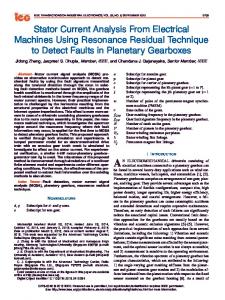
Fig. 4. Singular values of the PMSM model for !r (solid, dashed, dash–dotted, and dotted, respectively).
= {3, 0.5, 0.1, 0} p.u.
The sensitivity functions of the two cases are, hence, scaled by the machine transfer function matrix at the operating speed and zero speed, respectively. Let us make an evaluation in the frequency domain. As is a transfer function matrix, the gain is undefined. Instead, singular values have to be utilized; see [11], [13] and Section A of the Appendix. The singular values of for different are depicted in Fig. 4 for a PMSM having the parameter values and p.u. We can note the following characteristics. • For low frequencies ( ) and high speeds, IMC has significantly lower sensitivity than DIMC. Furthermore, the low-frequency sensitivity of IMC decreases with increasing speed. This is good, since the cross coupling increases with . IMC can, therefore, be expected to remove cross coupling better than DIMC. On the other hand, integral control action takes care of low-frequency cross coupling, so the difference between IMC and DIMC may not be overwhelming. • The drawback of IMC is the large sensitivity peak at , which is equal in magnitude to the sensitivity of DIMC at . This large peak is due to the attempt to cancel the machine dynamics (which are characterized by a complex pole pair, the imaginary parts of which follow the rotor speed [14]), and shows that oscillatory behavior can be expected at high speeds. The sensitivity analysis can be concluded by the following recommendation. DIMC is more desirable than IMC, as the sensitivity peak at is avoided. IMC has lower low-frequency sensitivity than DIMC, but the performance improvement is not expected to be overwhelming. Hence, IMC is of interest mainly not for direct implementation, but as a design method for standard PI controllers, with or without an inner cross-coupling removal loop added (DIMC).
(38)
where and
is the controller state vector, , is the inner feedback for cross-coupling removal.
A. Discretization Backward difference discretization [15] is suggested, which yields a simple algorithm: (39) (40) where time
is the sampling period and ).
the sampling instant (at
B. Inverter Saturation and Antiwindup A problem which has to be dealt with is that the output signal in practice must be limited, as the inverter will saturate whenever reaches the maximum available voltage. Let be the limited output:
(41)
However, only limiting the controller output signal will inevitably lead to poor performance. • Integrator windup results if the integration of the control error is not stopped when saturates. This is known to give large overshoots [16]. • The controller output limitation can be considered as a disturbance entering between the controller and the plant. IMC is sensitive to such disturbances, since the canceled plant dynamics are “activated” [7], [16]. This is undesirable also for DIMC, as the poles of the decoupled system are located close to the origin and will give rise to slow transients.
138
IEEE TRANSACTIONS ON INDUSTRY APPLICATIONS, VOL. 34, NO. 1, JANUARY/FEBRUARY 1998
Fig. 5. Vector block diagram of the DIMC current controller with antiwindup. (W = 0 for PI control.)
The above problems can be dealt with in the following way, which is known as back-calculation [16]. Step 1: At the sampling instant , compute the ideal controller output,
(42)
. This is the comand limit the signal, mand vector to the pulsewidth modulator (PWM) [1], [17]. Step 2: In order to avoid the problems discussed above, the saturation disturbance has to be “moved” from the controller output to the controller input. Hence, by inverting (42), compute the error signal which would yield : (43) Then use to update the controller state vector (i.e., the integrators): (44)
Fig. 6. Space vector modulation. T and Tsw are the sampling and switching periods, respectively.
C. Selection of the Sampling and Switching Frequencies It is important to select the sampling and switching frequencies high enough, so that the system performance does not degrade. Selecting the angular sampling frequency as at least 10 times the closed-loop bandwidth is a good recommendation [15]: (48)
If does not saturate, . The latter two equations can be slightly simplified by combining them as follows:
As for the switching frequency, two independent voltage space vectors can be generated per switching period using space vector modulation of a voltage-source inverter [1, ch. 4], as illustrated in Fig. 6. (This holds for the suboscillation PWM method as well.) The angular switching frequency should, hence, not be lower than half the sampling frequency. This yields
(45)
(49)
The controller matrices and can be simplified by making suitable approximations. We have
Using this formula and the relation , we can relate the switching frequency (in hertz) to the rise time:
(46)
(50)
and
(47)
This results in the block diagram depicted in Fig. 5.
A 1-ms rise time thus requires a switching frequency of at least 1.75 kHz. This is a low figure for insulated gate bipolar transistor IGBT and MOSFET inverters [17]; it is often desirable to switch faster for lower harmonic content and reduced acoustical noise. The recommendation obviously does not put excessive demands on the switching frequency. Neither is the recommended sampling frequency of 3.5 kHz too demanding.
HARNEFORS AND NEE: MODEL-BASED CURRENT CONTROL OF AC MACHINES
Fig. 7. PMSM simulation. Step responses for IMC (solid), DIMC (dashed), and PI (dash–dotted).
V. SIMULATION Consider a PMSM with the data in per-unit values and with a base frequency of 50 Hz, i.e., 314 rad/s. The permanent magnet flux p.u. and the maximum stator voltage p.u. The machine model is slightly incorrect: . From the machine model data we design a current controller for a closed-loop system rise time of 1 ms. Bandwidth Selection: The desired rise time corresponds to p.u., so the bandwidth should be selected as p.u. Sampling Rate Selection: The “10 times bandwidth” rule gives a sampling frequency of 70 p.u., i.e., 3.5 kHz. A one-sample delay is simulated to account for inverter and computational dead times. Evaluation: At p.u. and , we simulate the goes from 0.6 to 1.0 response to a setpoint step change; ms, while (see Fig. 7). p.u. and back again at At the first step, the inverter saturates during the transient, hence, the rise time is much longer than the desired. IMC is, as seen, slightly better than DIMC at removing the decoupling, which was predicted by theory. The difference is, however, not significant. Standard PI control gives a control error in which very slowly decays to zero.
139
Fig. 8. IM experiment. Step responses for DIMC.
rms value correspondence; p.u. corresponds to rated current and similarly for the stator voltage vector. A. Experiment 1 The motor is operated at no load at approximately 80% of rated flux and p.u. At ms, the setpoint for is stepped up 0.2 p.u. and stepped down again at ms. The setpoint for is held constant at 0.44 p.u. The step responses for DIMC are shown in Fig. 8. (It should be noted that has been adjusted vertically slightly, so that the step starts at 0.1 p.u. and the voltages and in stator coordinates are denoted as va and vb, respectively.) The step responses for PI are virtually identical and are not shown. This was to be expected due to the low rotor speed. The rise time is slightly shorter than the theoretical 0.88 ms. The settling time on the other hand is fairly long, which is an indication of slightly too low integral action. B. Experiment 2 The field is weakened ( p.u.) and the speed increased to 1.6 p.u. The same experiment is then repeated (see Figs. 9 and 10). This time, DIMC performs slightly better than PI. The slow decay of the control error in which was acknowledged in the simulation is also present here (although the error is not particularly large).
VI. EXPERIMENTAL RESULTS The DIMC algorithm is evaluated experimentally on an induction motor drive, the data of which are given in Section B of the Appendix. The IM is controlled using indirect rotor flux orientation [1, ch. 5]. It was found that p.u. is a good tradeoff between speed and robustness. A further increase was found to give too oscillatory a response. The nominal rise time is then ms. The control algorithm has a delay of one sampling period. Suboscillation method PWM generation is used, so the inverter is not utilized to its full capacity. Note in the following that the vectors are scaled for
VII. CONCLUSION In this paper, the concept of internal model control was applied to synchronous-frame current control for permanent magnet synchronous machines and induction machines. It was shown that the controller resulting from the IMC design method corresponds to two PI controllers with cross-couplingremoving integrators added. The additional cost of implementing IMC compared to PI control is negligible. An alternative structure, DIMC, using an inner decoupling loop and two outer standard PI loops was introduced as an alternative. DIMC is the structure preferable to use. Although IMC has
140
IEEE TRANSACTIONS ON INDUSTRY APPLICATIONS, VOL. 34, NO. 1, JANUARY/FEBRUARY 1998
TABLE I MACHINE DATA
Fig. 9. IM experiment. Step responses for DIMC.
in the implementation. With a state-of-the-art DSP, this is usually no obstacle, however, since trigonometric operations can be implemented using a lookup table or the CORDIC algorithm [18]. If coordinate transformations are still not desirable, the controller can be transformed to and implemented in stator coordinates, as shown in [19]. For further information, see [14]. APPENDIX A. Singular Values
Fig. 10.
IM experiment. Step responses for PI.
lower parameter sensitivity, there is also a risk for oscillatory behavior which is avoided with DIMC. The benefit of the IMC design method is that the controller parameters are expressed directly in the machine parameters and the desired closed-loop bandwidth. Hence, the design procedure is simple, and trial and error can largely be avoided. It should be stressed that, even if removal of cross coupling is not an important objective (see also [6]), IMC is still very useful for standard PI controller design. Rules for sampling and switching frequency selection were given and discrete-time implementation issues were considered. A backcalculation algorithm was suggested in order to avoid integrator windup (and, thus, degraded performance) when the inverter saturates at transients. We finally emphasize that the controllers are implemented in synchronous coordinates, which has been shown to yield the best performance among low-complexity current controllers [1, chs. 4, 5]. Therefore, coordinate transformations are needed
For a multivariable dynamic system, one can obtain a frequency function by substituting in any transfer function matrix, as for any single variable (scalar) transfer function. However, the gain is not as straightforward to express. It can be shown [11] that (51) where and are the minimum and maximum singular values. The singular values for a frequency function matrix are defined as (52) where is the th eigenvalue. There are as many singular values as there are inputs/outputs. (We consider square only.) It is, hence, not possible to talk about a fixed gain but a gain spread, bounded by and . The actual gain depends on the direction of the input vector . See also [13]. B. Data for Laboratory Induction Motor Drive 1) Machine: The data are given in Table I.
HARNEFORS AND NEE: MODEL-BASED CURRENT CONTROL OF AC MACHINES
2) Inverter: IGBT voltage-source inverter, 540-V dc link, 20-kW rated power, three-phase diode rectifier on mains side, analog suboscillation method PWM generation with 5.3-kHz switching frequency. 3) Digital Signal Processor: Texas Instruments TMS320C40 floating-point DSP, sampling frequency 5.3 kHz, DSpace development system on Pentium PC host. All algorithms are implemented in C code. Stator current and resolver signal sampling is made synchronously with inverter switchings, at the peaks of the PWM suboscillation triangular wave. This gives significantly reduced noise levels in the samples. C. A Sample Software Implementation of DIMC A C program implementing the DIMC control algorithm follows below. It should be self explanatory to anyone with some knowledge of programming. Constants are written in capital letters. Declarations of variables, constants, and functions are not shown. &
141
[4] R. D. Lorenz and D. B. Lawson, “Performance of feedforward current regulators for field-oriented induction machine controllers,” IEEE Trans. Ind. Applicat., vol. 23, pp. 597–602, July/Aug. 1987. [5] D.-C. Lee, S.-K. Sul, and M.-H. Park, “High performance current regulator for a field-oriented controlled induction motor drive,” IEEE Trans. Ind. Applicat., vol. 23, pp. 1247–1257, Sept./Oct. 1994. [6] J.-W. Choi and S.-K. Sul, “New control concept-minimum time current control in the three-phase PWM converter,” IEEE Trans. Power Electron., vol 21, pp. 124–131, Jan. 1997. [7] M. Morari and E. Zafiriou, Robust Process Control. Englewood Cliffs, NJ: Prentice-Hall, 1989. [8] I. Boldea and S. A. Nasar, Vector Control of AC Drives. Boca Raton, FL: CRC Press, 1992. [9] J. L. Thomas and M. Boidin, “An internal model control structure in field oriented controlled v.s.i. induction motors,” in Proc. EPE, Florence, Italy, 1991, vol. 2, pp. 202–207. [10] P. Vas, Electrical Machines and Drives: A Space-Vector Theory Approach. Oxford, U.K.: Clarendon, 1992. [11] J. M. Maciejowski, Multivariable Feedback Design. Reading, MA: Addison-Wesley, 1989. [12] W. Leonhard, Control of Electrical Drives. Berlin: Springer-Verlag, 1985. [13] L. Harnefors and H.-P. Nee, “On the dynamics of ac machines and sampling rate selection for discrete-time vector control,” in Proc. ICEM, Vigo, Spain, Sept. 1996, vol. 2, pp. 251–256. [14] L. Harnefors, “On analysis, control and estimation of variable-speed drives,” Ph.D. dissertation, Div. Electr. Machines and Drives, Dep. Elect. Power Eng., Royal Inst. Technol., Stockholm, Sweden, 1997. [15] R. H. Middleton and G. C. Goodwin, Digital Control and Estimation: A Unified Approach. Englewood Cliffs, NJ: Prentice-Hall, 1990. ˚ om and T. H¨agglund, PID Controllers: Theory, Design and [16] K. J. Astr¨ Tuning, 2nd ed. Research Triangle Park, NC: Instrument Society of America, 1995. [17] J. G. Kassakian, M. F. Schlecht, and G. C. Verghese, Principles of Power Electronics. Reading, MA: Addison-Wesley, 1991. [18] S. Y. Kung, VLSI Array Processors. Englewood Cliffs, NJ: PrenticeHall, 1988. [19] T. M. Rowan and R. J. Kerkman, “A new synchronous current regulator and an analysis of current-regulated PWM inverters,” IEEE Trans. Ind. Applicat., vol. 22, pp. 678–690, July/Aug. 1986.
Lennart Harnefors (S’94–M’98) received the M.S., Licentiate, and Ph.D. degrees in electrical engineering from the Royal Institute of Technology, Stockholm, Sweden, in 1993, 1995, and 1997, respectively. Since 1994, he has been with the Department of Electrical Engineering, M¨alardalen University, V¨aster˚as, Sweden, where he is a Senior Lecturer. He is also an Affiliate Senior Lecturer with the Division of Electrical Machines and Drives, Department of Electric Power Engineering, Royal Institute of Technology, Stockholm, Sweden. His research interests include circuits, systems, and control, particularly as applied to variable-speed drives.
-
REFERENCES [1] B. K. Bose, Ed., Power Electronics and Variable Frequency Drives. Piscataway, NJ: IEEE Press, 1996. [2] J. Holtz and S. Stadtfeld, “A predictive current controller for the stator current vector of ac machines fed from a switched voltage source,” in Proc. IPEC, Tokyo, Japan, 1983, pp. 1665–1675. [3] L. Zhang, R. Norman, and W. Shepherd, “Long-range predictive control of current regulated PWM for induction motor drives using the synchronous reference frame,” IEEE Trans. Contr. Syst. Technol., vol. 5, pp. 119–126, Jan. 1997.
Hans-Peter Nee (S’91–M’96) received the M.S., Licentiate, and Ph.D. degrees in electrical engineering from the Royal Institute of Technology, Stockholm, Sweden, in 1987, 1992, and 1996, respectively. Since 1988, he has been with the Division of Electrical Machines and Drives, Department of Electric Power Engineering, Royal Institute of Technology, Stockholm, Sweden, where he is a Research Associate and Director of the Permanent Magnet Drives Research Program. His research interests are permanent magnet and induction motor drives. Dr. Nee is the recipient of several awards, including a Best Paper Award at the ICEM’94 Conference.