_ x. ) is neglected. The time rate of change of the zone air temperature is given by: ..... supply air temperatures at Air Handler Unit (AHU) level with consideration ...
Fourth National Conference of IBPSA-USA New York City, New York August 11 – 13, 2010
SimBuild 2010
MODEL-BASED THERMAL LOAD ESTIMATION IN BUILDINGS
Zheng O’Neill, Satish Narayanan, and Rohini Brahme United Technologies Research Center East Hartford, CT 06108, USA
INTRODUCTION Model-based estimation approaches (Goodwin and Sin 1984, Dougherty and Astola 1999, Tanizaki 1996) have been widely applied in a variety of complex dynamical systems encountered in aerospace and process control applications. Model-based estimation is used here to provide real-time information about internal loads within a building that affects energy performance. The proposed estimation technique is built upon a reduced-order thermal network model and real-time data including temperatures and airflow rates from the Building Management System (BMS), considering uncertainties from sensor data and the model. A subset of real-time weather data is also incorporated into the estimation procedure. An Extended Kalman Filter (EKF) is used to estimate unmeasured states including room surface temperatures. The real-time load estimation will facilitate the understanding of building usage (i.e., occupancy, plug loads, lighting loads and process loads), and provide real-time load information where measurements are not available or are highly uncertain. The estimated load can also be used as inputs to diagnostic tools and to whole building simulation programs such as EnergyPlus (DOE 2010) and eQuest (eQuest 2010) as refinements to the input load profile.
This work focuses on the Classroom and Office Building (COB) at University of California at Merced Campus (UC Merced). Figure 1 shows the second floor plan in COB. This floor contains both offices and classrooms.
Figure 1 The second floor plan in COB The Extended Kalman Filter and the thermodynamic model were built in Matlab. Real time data from a database for the UC Merced, generated from Building Management System (BMS), were used for the study. Figure 2 shows the schematic of the proposed real time load estimator. This includes: 1) A reduced order state space thermodynamic model of specific zones, including internal and external zones, in the building based on non-linear algebraic and differential equations. 2) Utilization of EKF based on the model to estimate unknown states. 3) Testing and verification of estimation results with real time data and additional sensor data. Real time BMS data
Dynamic Reduced Order Building Model
Tamb Tosur 1/hoA
Extended Kalman Filter Based Estimator Time update
Rwin
Tisur Tzone 1/hiA Qstructure
R
Qsurfi
Qsurfo C
C
Measurement update
Internal loads (Plug load, lighting load etc.) 800 Qint (W) 600 Qint (W)
ABSTRACT Understanding and optimizing the energy performance of a building requires insights into the dynamics of thermal loads at a variety of spatial scales within the building. When available, sensors within the terminal units and indoor environment can provide useful information, but they can be grossly inaccurate when estimating loads over extended periods of time. Increasing the number of sensors or including more accurate sensors will help, but would increase the system complexity and lifecycle cost. The use of physics-based thermal balance models with measured data can provide more robust and accurate estimates of the loads. In this paper, a model-based approach is used to estimate zonal loads in a medium-sized commercial building and verified with measurements.
400 200 0
0
200
400
600
800
1000
1200
t (min)
Figure 2 Schematic of the real time load estimator
474
1400
Fourth National Conference of IBPSA-USA New York City, New York August 11 – 13, 2010
SimBuild 2010
APPROACH (METHODOLOGY) The EKF based on reduced order dynamic building models was used to estimate unmeasured variables and energy performance metrics. In this section, the thermodynamic reduced order model will be described first, followed by the implementation of EKF. Thermodynamic Reduced Order Model Physics based reduced order model The reduced order model is based on mass and energy balances in a given zone and will serve as the basis to estimate unmeasured internal loads. Two major assumptions were used in this simplified lumped model for a given zone: The zone is well mixed; Long wave radiation exchanges between surfaces are ignored. Energy balance equation of a zone with one lumped node can be described by:
m air _ zone C pa zone C pv
dTdt
zone
m air _ sa C pa T sa T zone m air _ sa C pv sa Tsa zone T zone Qint
N surface
Q
structure _ i
m inf C pa Toa T zone
N zone
m C T i
pa
zonei
T zone
i 1
i
m v C pv T zone
(1)
The internal water vapor generation rate ( m v ) is neglected since it is typically small in office and classroom buildings (as observed in UC Merced). The small heat transfer due to water vapor temperature difference between supply air flow and room air ( m air _ sa C pv saTsa zoneTzone ) is neglected. The time rate of change of the zone air temperature is given by: m air _ zone C pa
dT zone m air _ sa C pa Tsa T zone Qint dt
N surface
Q i
structure _ i
m inf C pa Toa T zone
(2)
N zone
m C T i
pa
zonei
T zone
N surface
Q
structure _ i
is the sum of the convective heat
i
transfer between the zone air and zone’s surface temperature;
N zone
m C T i
pa
zonei
Tzone is the sum of the heat
i 1
transfer due to interzone air mixing; m inf C pa Toa Tzone is the heat transfer due to infiltration of outside air. There is no information available about the humidity and water vapor generation at the zone level in the selected building. Therefore, the issues related to water vapor and humidity were not considered. A circuit-equivalent 3R2C thermal network of building zones shown in Figure 3 was used. Existing whole building simulation models such as EnergyPlus (DOE 2010) and eQuest (eQuest 2010) are typically computationally intensive and can be complex in the number of parameters needed. Since a large number of parameters are needed as inputs for simulation, the process of collecting and inputting physical descriptions becomes time consuming. Moreover, the states, which are required for estimation, cannot be accessed easily in these simulation programs, which are important for the purpose of estimation. 3R2C models as shown in Figure 3 have been successfully used to simulate the building envelopes for transient building load prediction (Braun and Chaturvedi 2002) and control algorithms testing (ASHRAE 1997). The nodal placement of the 3R2C model can be obtained by matching the theoretical frequency response characteristics of the building envelope with the frequency response characteristics of the simplified model using genetic algorithm (Wang and Xu 2006).
i 1
where, mair_zone (kg) is the air mass for a given zone; Cpa (J/kg.°C) is the specific heat capacity of dry air, Cpv (J/kg.°C) is the specific heat capacity of water vapor; Tzone (°C) is the zone temperature, Tsa (°C) is the supply air temperature, Toa (°C) is the outside air temperature; m air _ sa (kg/s) is the supply air mass flow rate,
v m inf (kg/s) is the infiltration mass flow rate, m
dQint 0; dt
(kg/s) is the internal water vapor generation rate; Qint (W) is the sum of the convective internal loads, which is assumed to be constant or slowly varying in comparison to other variables:
Rwin
Tamb Tosur 1/hoA
Tisur Tzone 1/hiA Qstructure
R
Qsurfi
Qsurfo C
C
Figure 3 A circuit-equivalent 3R2C thermal network model The heat balance equations for outside and inside surfaces are given by: C
475
dTosurf dt
ho A Tamb Tosurf
Tisurf Tosurf R
Qsurfo
(3)
Fourth National Conference of IBPSA-USA New York City, New York August 11 – 13, 2010
SimBuild 2010
C
dTisurf dt
hi A Tzone Tisurf
Tosurf Tisurf
Q surfi
R
(4)
The heat balance equation for the zone air node is given by: (T Tzone ) Qstructure hi A(Tisuf Tzone ) amb Rwin
(5) The thermal resistance, R , and capacity, C , are defined as: C p lA l , C (6) R 2 kA where, Tosurf (°C) is the outside surface temperature , Tisurf (°C) is the inside surface temperature, Tamb (°C) is the ambient temperature; Qsurfo (W) is the outside surface solar radiation heat flux (long wave and short wave), Qsurfi (W) is the inside surface solar radiation heat flux, Qstructure (W) is the heat flux from structure (building envelope) to the zone air node; ho (W/m2.°C) is the outside surface heat transfer coefficient, hi (W/m2.°C) is the inside surface heat transfer coefficient; A (m2) is the surface area, l (m) is the thickness of surface; K (W/m.°C) is the thermal conductivity of surface, Cp (J/kg.°C) is the specific heat of the surface, ߩ (kg/m3) is the density of the surface materials; Rwin (°C/W) is the window resistance including both inside and outside films. A room on the second floor is considered with four walls and the assumption of adiabatic boundary conditions for the floor and the ceiling. Equations (1b), (3), (4) can be rewritten in an ordinary differential equation (ODE) format as: dTzone m air _ sa Tsa T zone Qint dt m air _ zone m air _ zone C pa j
dT
dt j dTisurf
dt
[h A T T j
j
j osurf
[hi A T zone T j
j
j isurf
j isurf
T
T
osurfw
Rj j j Tosurf Tisurf
Rj
Q
j surfo
Q
]/C
j surfi
]/ C
dQint 0 dt
where, j w, n, e, s is the index for surrounding zones: west, north, east and west; A (m2) is the surface area; hi (W/m2.°C) is the internal surface convective heat transfer coefficient; ho (W/m2.°C) is the
(
m sw
(8)
) m sw
The optical parameters used in this work are listed in Table 1. We assume that solar transmissivity (τ) is zero for the opaque construction. Table 1 Optical parameters for the wall and window Solar absorptivity (ε) Solar transmissivity (τ) Solar reflectivity (α)
j
j
A
m
where, m n is the index for surfaces including wall, roof and windows; k is the index for the given interior surface; Htot (W) is all solar radiation transmitted from the exterior to the room, which is calculated from whole building simulation program; A (m2) is the surface area; is the solar absorptivity; is the solar transmissivity.
(7)
j
k k sw sw N nf
m 1
j
win
j o
k q room (1 swfloor ) H tot
hi j A (Ti j T zone ) (T T ) amb j zone m air _ zone C pa R j
j osurf
external surface heat transfer coefficient; T j (°C) is the zone temperature from surrounding zones (west, north, east and west); Qint (W) is defined as the lumped load which includes equipment load, lighting load and occupant load (convective part), infiltration load, and load due to interzone air exchange. In this work, the total solar heat flux on the exterior wall surface is used after the shading and solar energy transmitted through window are taken from a whole building simulation model of the building (e.g., eQuest model or EnergyPlus model). To compute the solar heat flux for the room interior surfaces, we assume that all solar radiation (direct and diffuse) that enters the room first hits the floor, and that the floor diffusely reflects the radiation to all other surfaces. Multiple reflections are neglected. Area-weighted solar distribution factors instead of view factors are used to compute the solar heat flux on the given interior surface k:
Wall 0.7 0 0.3
Window (inside) 0.06
0.697 0.243
State Space Formulation The state space formulation will be illustrated for multiple zones only. Figure 4 shows the layout of multiple zones on the second floor of COB. There are 7 zones: Office: Zone 1, Zone 2, Zone3 Classroom: Zone 4, Zone 6 Corridor: Zone 5 Computer lab: Zone 7
476
Fourth National Conference of IBPSA-USA New York City, New York August 11 – 13, 2010
SimBuild 2010
7 zones 33 surfaces 82 states
1
2
3 4
7
5 6
Figure 4 Multiple zones on the second floor In this case, data is received from a number of different sensors, and we assume that they are independent. For the multiple observation streams, the system model has the form: X f ( x, u ) (9) y k g k ( x)
The state space formation for this multi-scale system with seven zones can be described as: x j
hjAj h j A j 1 j 1 j o j j j x osurface j j x isurface T R C R C Cj C
x j
osurface
isurface
o
hjAj i
Cj
x k
T _ zone
xk
T _ zone
osurface
Cj
h j Aj 1 1 j x j j j x j osurface j j R C R C C i
isurface
Qj
(10)
isurface
Cj
k m k M sa
A
1 m R m 1 xk M k c pa
Nwindows m
h
m w ,e ,n , s ... k pa
M c
m i
Nwindows
j out
Qj
x
k Q int
M k c pa
m T k
k
sa
sa
M k c pa
m 1
win
T _ zone
1 Rm
M k c pa
win
A
m
m w,e ,n , s ... k
m
m
i
isurface
h x
comparison to other variables:
where, j is the index for surfaces including wall, roof and ceiling; k is the index for the given zone; Nwindows is the total numbers of windows in a given zone; ݔ௦௨ (°C) is the outside surface temperature for a given surface j; ݔ௦௨ (°C) is the inside surface temperature for a given surface j; ܳ௦௨ (W) is the outside surface solar radiation heat flux for a given surface j; ܳ௦௨ (W) is the inside surface solar radiation heat flux for a given surface j; ̴்ݔ ௭ (°C) is the zone temperature for a given zone k; M (kg) is the air mass for a given zone k;
ೖ ௗ௫ೂ
The state vector is:
ௗ௧
≈0.
k xTk _ zone Tzone j j x Tisurface (11) Zone k isurface j x osurface T j k osurface k xQ int Qint
Zone1 Zone 2 X . k Zone k 7
M c pa
Tamb
Cpa (J/kg.°C) is the specific heat for the air; Tamb (°C) is the ambient temperature; ܶ௨௧ (°C) is the neighboring zone temperature for a given surface j; ܥ (J/K) is the themal capacity for a given surface j; ܴ (°C/W) is the thermal resistance for a given surface j; ℎ(W/m2.°C) is the internal surface convective heat transfer coefficient for a given surface j; ℎ (W/m2.°C) is the external surface convective heat transfer coefficient for a given surface j; ̇ (kg/s) is the supply air flow rate for a given ݉ ௦ zone k; ܶ௦ (°C) is the supply air temperature for a given zone k; ܣ(m2) is the area for the given surface j; ܴ௪ (°C/W) is the thermal resistance for a given window m. ݔொ ௧ (W) is the lumped load for a given zone k, including equipment load, lighting load and occupant load (convective part), infiltration load, and load due to interzone air mixing. Assume ݔொ ௧ to be constant or slowly varying in
There are 33 surfaces in the 7 zones. Therefore, this system has 82 states, which includes 7 zone temperatures, 66 surface temperatures, and 7 lumped loads. The outputs from the measurements are the measured room temperatures. So, the output equations become:
yk Ck X Where,
(12)
C zeros(1,82) k
(13)
C 1 (1) 1; C 2 (11) 1; C 3 (25) 1; C 4 (37) 1 C 5 (47) 1; C 6 (59) 1; C 7 (75) 1
For
this
dynamic
system,
U uzone1 u zone2 u zone3 u zone4 u zone5 u zone6 u zone7
is the input vector. Each zone has supply air flow rate ̇ ), supply air temperature (ܶ ), and surface heat (݉ ௦ ௦ k flux (ܳ௦௨ and ܳ௦௨). Y Tzone is the history of room temperatures from sensor measurements for a given zone k.
477
Fourth National Conference of IBPSA-USA New York City, New York August 11 – 13, 2010
SimBuild 2010
for the second floor of the COB with data acquired in August 2007 are presented.
Estimation with Extended Kalman Filter (EKF) The Kalman Filter (KF) approach provides an efficient recursive means to estimate the state of a process, in a way that minimizes the mean squared error. The filter can be used to estimate past, present, and even future states. The EKF is a filter to handle non-linear problems, which linearizes the estimation by using the partial derivatives of the process and measurement functions. Details about KF can be found from classic control theory textbooks. Figure 5 illustrates the operation of the EKF (Welch and Bishop 2006).
xˆ
Measurement update
xˆ
(Correct) Time update
Find constrained estimates
(Predict)
~ x Figure 6 Recursive operation of KF with constraints
Covariance For load estimation in buildings, we made assumptions for the process noise covariance Q, measurement noise covariance R, and initial estimate error covariance P0: Q=1* I (10, 10) Q (10, 10) =1*10^5 R= 1 P0=1000*I (10) RESULTS AND ANALYSIS In this section, estimation results from an interior room, an exterior room and a multi-zone representation
Zone Temp T ( C) T (C) T ( C)
T (C)
78 76 74 80
77 76 75
75
Supply Air Flow Rate CFM
76 74 72
T ( C)
West Zone Temp
80
200
North Zone Temp
East Zone Temp
100 0
T (C)
Figure 5 Operation of the Extended Kalman Filter In this work, an EKF was used to estimate the state X using available sensor data for a given period. Knowledge of variance of modeling error and sensor noise is required for designing the filter. Matlab Kalman Filter tool box was used. In our problem, there are some soft and hard constraints for the KF estimation. The constrained KF is derived by directly projecting the unconstrained state estimate x onto the constraint surface. Figure 6 shows recursive operations of KF with constraints. Details about the fundamental designs for the EKF with parameter constraints can be found from the literature (Simon 2006).
Interior Zone (Room-248) The location of an interior zone (Room-248) is highlighted with red in Figure 1. Figure 7 shows all the post-processed input data to the estimation model of Room 248 in August, 2007. All the data are interpolated to a sampling time of 2 minutes. In the post-processing, negative air flow rates are reset to zero with consideration of VAV damper positions. Currently, COB BMS does not have points for supply air temperature at zone level. The cold deck supply air temperatures at Air Handler Unit (AHU) level with consideration of heat loss/addition are used as approximations of zone level supply air temperature. In this study, 5°C temperature rise is used, which is justified by additional portable sensors measurement (see section verification). In August 2007, the supply fan in hot deck was always off. Therefore, we assumed that supply air was only from the cold deck during this month.
Supply Air Temp
75
West Zone Temp
60 40 0
1
2 Time (mins)
3
0
4 x 10
4
1
2 Time (mins)
3
4 x 10
Figure 7 Post-processed input data for Room 248 Figure 8 shows the estimated load together with measured zone temperature and supply air flow rate in this interior room for a day. The lumped estimated load includes load from internal lighting, equipment, people and inter-zone mixing. The correlation of estimated loads with ventilation suggests that the estimated values are reasonable. The estimation captures the daily (daytime vs. nighttime) and weekly (weekday vs. weekend) variation for the estimated loads as shown in Figure 9. Exterior Zone (Room-229) The location of an exterior zone (Room-229) is highlighted with blue in Figure 1. Figure 10 shows estimated lumped loads for an exterior zone (office 229). The lumped load in this zone includes internal lighting load, plug/equipment load, occupant load and infiltration load. The estimation captures the daily (daytime vs. nighttime) and weekly (weekday versus weekend) variation for the lumped loads as shown in Figure 10. From the asbuilt drawings and eQuest/EnergyPlus input files, the maximum internal loads for this office zone is 482 W
478
4
Fourth National Conference of IBPSA-USA New York City, New York August 11 – 13, 2010
SimBuild 2010
(lighting: 120W, equipment: 222W, people: 70×2=140 W – assume two people in the room and 70W sensible load per person). The majority of the estimated lumped load is less than 482W. The possible reasons for the lumped load estimates being greater than the maximum internal loads are: Lumped estimated load includes infiltration load; The solar heat flux as inputs to the estimation load are calculated from eQuest model based on TMY2 solar data instead of real time solar data. TR (C)
26 Sensor Data
25 24 23 0
200
400
600
800
1000
1200
1400
Qint (W)
Qint (W) 500
0
0
200
400
600
800
1200
1400
Supply Air Flow Rate
200 CFM
1000
100 0
0
200
400
600 800 Time (mins)
1000
1200
1400
Multiple Zones A simplified model to estimate loads for multiple zones on the second floor was developed based on the building 3R2C thermal network model described in this paper. The EKF procedure was used to estimate the unknown states, in particular the lumped loads. Average room temperature from individual rooms in a given zone was used to represent the zone temperature. Total sum of supply air flow rate from individual rooms in a given zone was used for the zone supply air flow rate. The plots in Figure 11 show the estimation results in August 2007 for the 7 zones illustrated by the floor plan in Figure 4. The estimated lumped load includes lighting load, equipment load, occupant load, infiltration load (for exterior zones), and loads due to interzone air mixing. The estimated load (yellow line) for the computer lab is always greater than zero, which empirically confirms the 24-hour operation schedule in the lab. The estimated load for zone 6 increased significantly in the last week of August. This is because student classes started that week and the rooms were heavily used. Estimation error is also affected by solar heat flux calculations as discussed before. x 10
Figure 8 One day estimation results for Room 248 TR ( C)
Z1Q Z2Q Z3Q Z4Q Z5Q Z6Q Z7Q
Office: Zone 1, Zone 2 Zone3
4.5
Sensor Data
26
4
Classroom: Zone 4, 6 4
1
2
3 4
24
7
5
Hallway: Zone 5
6
Computer lab: Zone 7
Qint (W)
1440
2880
4320
5760
7200
8640
10080
Qint (W) 500
0
Weekend 0
1440
2880
4320 5760 Time (mins)
7200
8640
10080
Estimated Load Q (W)
3.5
0
TR (C)
2
1 0.5
30 Sensor Data
28
0
26 24 0
Qint (W)
2.5
1.5
Figure 9 One week estimation results for Room 248 in August 2007
1000
2000
3000
4000
5000
6000
600
7000 Qint (W)
0
0.5
1
1.5
2 2.5 Time (mins)
3
3.5
4 x 10
4
Figure 11 Estimated loads for multiple zones on the second floor in August 2007 VERIFICATION
400
Weekend
200 0
1000
2000
3000
4000
5000
6000
7000
200 Supply Air Flow Rate CFM
3
100 0
0
1000
2000
3000 4000 Time (mins)
5000
6000
7000
Figure 10 Five-day estimation results for Room 229 in August 2007
Simulation Based Zonal Load Estimator Validation Simulated data from the EnergyPlus COB model, developed by Lawrence Berkeley National Laboratory (Black 2009) was used to test the accuracy of the load estimator. Outputs from the EnergyPlus including zone temperatures, supply air flow rates, and supply air temperatures for the room 250 on the second floor with a given internal heat gains profile are treated as inputs (i.e., from sensors) in the estimator. Since the reduced order model in the estimator does not account for internal thermal mass sources such as furniture, to 479
Fourth National Conference of IBPSA-USA New York City, New York August 11 – 13, 2010
SimBuild 2010
enable a clear comparison, the internal thermal mass modeling in the EnergyPlus is not used. Eplus Input Load Estimated Load
Q(W)
400 200 0 0 Difference(W)
Figure 14 shows the comparison between room air temperatures from the portable sensor and BMS for the same period. The temperature readings from the portable sensor are higher than that from BMS because the portable sensor was installed near the lighting fixture. Therefore, the room temperatures from BMS are used for the estimation. The other variables from BMS used as the inputs to the estimator are supply air flow rates and room temperatures in the surrounding zones. Solar data used in the estimator are taken from the eQuest output.
200
400
600
800
1000
1200
1400
200
400
600 800 Time (mins)
1000
1200
1400
200 0 -200
Room Temp Room 229 DDV 242 28
R241
R250
R248 R229
R207 R205 R203
Figure 13 Floor plan for the portable sensor deployment
BMS Data Portable Sensor Data
27 26 25 24 23 22
0
1000
2000
3000
4000
5000 6000 Time (2 mins)
7000
8000
9000
10000
Figure 14 Comparisons of room temperatures from the portable sensor and BMS Figure 15 shows the comparisons between supply air temperatures from the portable sensor in Room 229 and supply air temperatures at AHU level from BMS for the same period. During the occupied period, supply air temperature readings from the portable sensor are about 5 °C higher than that from the AHU level due to the heating additions in the duct. AHU CD Temp from BMS Supply Air Temp from Portable Sensor
25 Temperature (C)
Sensor Based Verification 14 portable sensors (Onset 2010) were deployed in 7 rooms in COB. Two portable sensors were installed in the individual room marked by red rectangle, as shown in Figure 13. One portable sensor was close to the supply air diffuser, which is intended to measure supply air temperature and humidity. The second portable sensor was placed in the middle of room to measure room temperature, humidity and lighting intensity. Real time data including room air temperature, room air humidity, supply air temperature (at zone level) and lighting intensity were sampled every two minutes from May 28th to June 16th, 2009 with the portable sensors.
Room Temperature ( C)
Figure 12 Comparison results for testing /validation of load estimator in a weekday for room 250 Figure 12 shows comparisons between the estimated internal load and the EnergyPlus input internal heat gain profile for a weekday in the room 250. For the most part, the estimated load matches the EnergyPlus input profile well; in particular, 93% of the time the estimated load is within a ± 10% error band. More simulation based validation case studies can be found from the related report (Apte et al. 2010). The possible reasons causing the differences are: Reduced order 3R2C thermal network model to model the building envelope heat transfer vs. CTF (Conduction Transfer Function) model in Energy Plus; The reduced order model does not consider the long wave radiation heat exchanges.
20
15
10
1000
2000
3000
4000
5000 6000 Time (2 mins)
7000
8000
9000
10000
Figure 15 Comparisons of supply air temperatures from the portable sensor in Room 229 and AHU cold deck supply air temperatures from BMS Figure 16 illustrates the estimated loads for an interior room – R248 from June 1st to June 15th, 2009. The profile for estimated loads (blue line), including lighting load, plug load, and load due to interzone mixing, follows the variation of the lighting intensity (red line) measured by the portable sensor (Figure 17). The maximum loads from occupants, lighting and equipments, taken from EnergyPlus input file, are plotted with the estimated load. In this interior room without daylighting, we converted lumens to watts by assuming a luminous efficacy of 85 lumen/W, and that the portable sensor is only exposed to 75% of light’s output (in lumens) in the room based on position. 480
Fourth National Conference of IBPSA-USA New York City, New York August 11 – 13, 2010
SimBuild 2010
500
or known changes in heat inputs (e.g., controlled electric heaters).
Qint (W) Lighting Q Based On Lumen
Max EQP+LTG+OCC =475W
ACKNOWLEDGMENT
Load (W)
400
The funding provided by United Technologies Research Center for this work is greatly appreciated. The authors are grateful to John Elliott from UC Merced for providing access to the data which was acquired with funding support from DOE under contract DE-AC02-05CH11231.
300 Max EQP+LTG=233 W 200 Max EQP=152 W 100
Max LTG= 82 W
REFERENCES 0 0
0.2
0.4
0.6
0.8
1 1.2 Time (mins)
1.4
1.6
1.8
2 4
x 10
Figure 16 Estimated loads for an interior room R248 from June 1st to June 15th, 2009 400 Qint (W) 2
Lighting Intensity (lum/ft )
Load (W)
300
ASHRAE 865 RP Final Report. 1997. A Standard Simulation Test bed for the Evaluation of Control Algorithms and Strategies. Braun, J. and Chaturvedi, N. 2002. An Inverse Graybox Model for Transient Building Load Prediction, HVAC&R Research. 8 (1):73–99. Black, D. 2009. Personal communication.
200
DOE. 2010. http://apps1.eere.energy.gov/buildings/energyplus/ 100
0 2880
Time (mins)
4320
Figure 17 Estimated loads variation vs. measured lumen variation in an interior room R248 for one day CONCLUSION This work developed and demonstrated a model-based estimation thermal load technique for buildings. An approach combining models with sensors was proposed and implemented with measurements in a medium sized commercial building. A lumped and reduced order model of room temperature dynamics was developed. Testing results show that an Extended Kalman Filtering framework works well to dynamically estimate building loads. Accuracy of the load estimator depends on input parameters such as envelope thermal properties (e.g., thermal resistance and capacity) and time series input from BMS such as supply air flow rates and temperatures. Future efforts are recommended in the following directions: 1) Dynamic models could be improved by integration of solar heat flux calculation based on real time solar data instead of using output from a whole building simulation program. 2) Collect more real time data such as solar data and zonal supply air temperature. 3) Use the estimated load to refine the input load profile to energy simulation programs. 4) Develop methodologies to connect zonal load profiles/estimation to whole building performance and operational problems. 5) Calibrate the estimator with a known heat source
Dougherty, E. R. and Astola, J. T. editors. 1999. Nonlinear Filters for Image Processing. SPIE/IEEE Series on Imaging Science & Engineering. SPIE Optical Engineering Press, Bellingham, WA. eQuest. 2010. http://www.doe2.com/eQUEST/ Goodwin, G. C. and Sin, K. S. 1984. Adaptive Filtering Prediction and Control. Prentice Hall, Englewood Cliffs, NJ. Apte, M.G., Berkeley, P., Black, D.R., Price, P.N., Najafi, M., Narayanan, S., Brahme, R., O’Neill, Z., Sevilla, E., Spears, M., Elliott, J., Erickson, V., Kamthe, A. and Piette, M. A. 2010. Real-Time Visualization of Energy Performance in Buildings. DOE report: DE-AC02-05CH11231. Onset. 2010. http://www.onsetcomp.com/ Simon, D. 2006. Optimal State Estimation: Kalman, H Infinity, and Nonlinear Approaches. John Wiley &Sons. Tanizaki, H. 1996. Nonlinear Filters. Springer-Verlag, Berlin, second edition. Wang, S. and Xu, X. 2006. Simplified Building Model for Transient Thermal Performance Estimation Using GA-based Parameter Identification. International Journal of Thermal Sciences. 45 (2006): 419–432. Welch, G. and Bishop, G. 2006. An Introduction to the Kalman Filter. http://www.cs.unc.edu/~welch/kalman
481