"Model Checking", In Wiley Encyclopedia of Computer Science and ...

1904

MODEL CHECKING

MODEL CHECKING INTRODUCTION Model checking was proposed in the 1980s independently by Clarke and Emerson (1) and by Quielle and Sifakis (2). It is a notion taken from mathematical logic, which means the process of testing the correspondence between a logical formula against a mathematical structure (i.e., a model). This notion is adopted in the study of software and hardware systems to describe the process of validating that a description of systems satisfies a given formal specification. In a broader view, this means the automatic or semiautomatic verification of systems. As such, model checking is an important member of the family of formal methods (3, 4), together with testing and deductive verification, which are all aimed at improving the reliability of systems. Model checking (5) does not attempt to validate that a system is error free. This task is obviously impossible, as automated verification systems may contain errors themselves. Another difficulty is having an informal, incomplete, or incorrect specification against which the system is compared. Finally, verifying a system directly requires interfacing with it, which may be of limited availability (e.g., consider the physical limitations of measuring some properties of a system, including accuracy, speed and physical measuring errors) and can be highly time consuming.

Wiley Encyclopedia of Computer Science and Engineering, edited by Benjamin Wah. Copyright # 2008 John Wiley & Sons, Inc.

MODEL CHECKING

For these reasons, model checking has a more modest goal; it assumes an available mathematical model of a system, which is represented in computer memory, and a given formal specification, in some logical formalism. The goal of model checking is then limited to comparing the given model with the given specification. This consistency checking is performed in an algorithmic way, which leaves some difficulties. First, the theory of computability (6) provides the inherent problem that, in general, system verification can be undecidable (computability theory shows that termination of programs is, in general, an undecidable problem) or intractable (i.e., of very high complexity). Thus, one main challenge of model checking is to identify large classes of verifiable models and specification formalisms with attainable algorithmic complexity. Because model checking is desirable even when it is, in general, undecidable or inherently complex, a related challenge is the generation of effective heuristics that work efficiently in many situations, e.g., for the verification of Java programs (7). The systems to be verified can greatly differ from each other. We list some main characteristics that systems can have: Finite versus Infinite Systems. Automatic verification was initially limited, for decidability considerations, to finite state systems. Later, research has allowed some restricted classes of infinite state systems to be verified (8), which includes stack machines (i.e., finite control with recursion); real-time systems with multiple clocks that can be set, reset and compared with a constant; and hybrid systems with differential equation-based parameters and systems with lossy channels. Sequential versus Concurrent Systems. Verification complexity increases exponentially with the number of concurrent threads. Although even purely sequential systems may be sometimes difficult to verify, concurrency, where control of different parts of the system can reside independently and simultaneously in different locations, poses additional challenges. Deterministic versus Nondeterministic Systems. Sequential systems are often deterministic, in the sense that the next action to be performed by the system is uniquely defined by the current state. Concurrency usually results in nondeterminism, because the duration of actions in concurrent components is not known or abstracted away; thus, depending on speed, different continuations to the current ongoing execution can occur. However, nondeterminism can also result in from having an interaction with an environment that must be encapsulated in the modeling of the system. Software versus Hardware. Hardware systems are by nature finite state systems, and they are usually much smaller than software systems (e.g., consider the number of states in a small program with only three 32-bit variables). Hence, model checking is used much more frequently in the hardware industry (9) than in the software development industry (10). Synchronousversus Asynchronous Systems. Hardware systems are often synchronous, designed around a

1905

single clock that controls the change of all gates and registers. Software systems are often built from different components (which may be distributed in different locations), which progress independently and asynchronously, each with its own speed. MODELING SYSTEMS Because we do not model check systems directly (but see Ref. 11 for a direct yet costly approach), we first need to model them. Modeling can be done automatically or manually. A model may not reflect correctly the behavior of the verified system; modeling errors do occur often. Even if done automatically (e.g., using a compiler that generates the description of the system), errors related to mistakes in the compiler or some unclear or nonstandard semantic definitions of the system may occur. A model is characterized by the set of configurations that the considered system can assume, which are called the states of a system. A state is defined over a set of variables. This set includes program and control variables (in case of a software system) or gates and register values (in case of a hardware system). A state may also include additional components of the system, such as the contents of inter process communication channels. Roughly speaking, it can be considered as the snapshot of the system in a point of its evolution. The future behavior of a system solely depends on the current state and not on the history of the computation. The system evolution is represented in the model by atomic changes, which are performed by transitions or actions, between one state and a following state. The atomicity level of a transition is fixed by the level of detail in which we want to describe the system. Atomic actions are also related to the effect of asynchronous concurrency; we usually want to enforce that any pair of actions from different concurrent components will behave in a commutative way. That is, executing them concurrently has the effect of applying them to the current state in either order. If this is not the case, then the granularity level of modeling is wrong. As a trivial example, consider two processors that access mutual memory location 344, trying to increment it by 1. Let us suppose that in modeling we attempt to describe some high level action, as m344:=m344+1, and that it is implemented in machine code not as an atomic action. We first need to read the value of memory location 344 into a register and then increment it returning the result value. The result may be different from the one obtained by incrementing location 344 twice. Consider the case where firstly both processes read the location into internal registers, then they increment their internal registers and finally they write back to memory. Thus, our model with such an atomic action is erroneous, as it may lose some possible behaviors of the modeled system. Using atomic actions that are too small, however, may result in needless details and increase in the complexity of the verification. A transition a is enabled in a state s only if the system can progress by executing a from s. The system is deterministic if executing a from s, when enabled, results in a single state s0 . A state s from which no transition is enabled is called final.

1906

MODEL CHECKING

Under the commonly used interleaving semantics, an execution (or execution sequence) is a finite or infinite alternating sequence of states and transitions r ¼ s0 a0 s1 a1 s2 . . .. The state s0 is an initial state of the system (i.e., a state from which the system can start). (Often, the execution of a system may start from different initial states, but this situation can be reduced to the case of a single initial state, by adding an additional, unique, initial state, which precedes all the other previously considered initial states.) Furthermore, for i
0, si+1 is obtained by executing some atomic action a from si. We require that an execution will be maximal (i.e., either an execution ending in a state where no transition is enabled, or an infinite execution). Sometimes, to deal with only one type of execution, we may coerce a finite execution s0 a0 s1 a1 s2 . . . an1 sn to become infinite by appending infinitely many occurrences of a dummy no_op operation. Because the effect of concurrently executed actions is commutative, the actions are modeled (‘‘interleaved’’) as appearing one after the other in some arbitrary order, which generates different executions. An execution can be embedded within a graph structure, namely the state space of the system, with nodes that are the reachable states of the systems and edges that correspond to the transitions from one state to its successor, because of the execution of an atomic action. An execution is then a path of such a graph. In modeling, one can describe this using an unfolding of the graph, which is a (possibly infinite) tree obtained using a breadth first search of the graph that starts from an initial node and replicates nodes each time they occur in the search without stopping at any node that has already occurred. In such an unfolding, one can observe the branching points where one execution departs from another. The difference between viewing the behaviors of a system using the set of all executions or using a single branching structure has been the ground for intensive and inconclusive debates over the last couple of decades (12). Another model for concurrency represents executions as a partial order structure among the executed events (13, 14). In this case, events that share the same concurrent process are always totally ordered, whereas independently executed events may be unordered. Local states (related to a single process or to several processes that participate in a single action) are associated just before and after each action. States in the sense defined above, which are also called in this context global states, can be formed by combining local states of all the different processes in a consistent way. Each global state s partitions the execution into two sets of events: the events that already occurred (before s) and those that did not occur before s. It is sometimes argued that this model provides some more intuitive representation of concurrent executions. The interleaving model and the partial-order model are closely related, because one can obtain from each partial order execution its linearizations, which are interleaved executions (completing the partial order into a total order, where each event occurs after some finite number of events). In this case, an important equivalence relation exists between executions that are linearizations of the same partial order execution. Specifications that require the partial order semantics are not very frequently used.

Furthermore, the mathematical machinery of the interleaving semantics is easier to use and understand; hence, this model is more popular. In concurrent systems, one often imposes fairness constraints (15), which limit the executions. Such constraints are required to disallow executions that are physically unreasonable, for example, where some process can progress, but is always overtaken by another concurrent process that does not interact with it. Several standard fairness assumptions can be used for concurrent systems. For example: Weak action fairness. We do not allow an execution where from some state an action is enabled forever but is never executed. Strong process fairness. We do not allow an execution where from some state some process has infinitely many states in which at least one of its actions is enabled but is never executed. Correct modeling is an engineering practice. One cannot guarantee that a system is correctly modeled (in the same way that one cannot guarantee that physics modeling is accurate). The correct choice of model, granularity, and fairness assumptions can affect correctness of applying model-checking techniques. Hence, as a safety measure, model checking results must be accompanied with testing against the actual system. This concept is especially true when model-checking results point to incorrectness and provide counterexamples to the checked property. In fact, a model may include more behaviors of the concrete system, some of which are not allowed by the concrete system. Therefore, a counterexample could be a false negative.

SPECIFICATION FORMALISMS In model checking, a model of the system is verified against its specification. The specification may be considered as a contract between the users of the system and the developers. As such, it must be uniquely readable and have an agreed semantics. To apply an algorithm for checking the consistency between the system description and the specification, the specification must be machine readable. For sequential systems, which take some input at the beginning of the execution and provide some calculated output on termination, the specification is usually given as a condition on the input, and a relationship between the input and the output values. In the more involved case of concurrent systems, frequently we are also interested in the behavior of the system throughout the execution, not just at its beginning and end points. In particular, in some concurrent systems, termination is not scheduled for a particular time and may even be considered a failure (consider, e.g., internet services). This result calls for the use of temporal logic (12, 16–18), which can relate different states of the system throughout its execution. Properties to be verified are in general classified into two categories: safety properties, which state that ‘‘nothing bad’’ will will happen during the execution of a system and liveness properties, which stipulate that ‘‘something good’’ will eventually happen during the execution of a system.

MODEL CHECKING

Alpern and Schneider (19), who defined a property of a system as a set of executions, provide a more formal characterization of safety and liveness as follows: 



A safety property is a set of executions that satisfies the following closure property: If there is a sequence r such that every finite prefix of r can be completed into an execution in the set, then r is also in the set. A liveness property is a set of executions such that each finite execution can be completed into an execution in this set.

Alpern and Schneider also show that every property is an intersection of a safety and a liveness property. Other classifications of properties are used (20). A variety of specification formalisms are available. In general, the debate on which one to choose for specifying the properties of a given system is far from being settled. The main parameters in which specification formalisms for systems differ are: Complexity. Given a class of models (e.g., finite state systems represented using state space graphs), it is possible to analyze the complexity of verifying a system against its specification. Formalisms are often designed with the goals of allowing intuitive and compact representation of properties. However, formalisms that exhibit more compact representations of properties often require a decision procedure of higher complexity. Expressiveness. Various formalisms have different limitations on the ability to specify properties of the system. Extending the expressive power of a formalism often comes at the cost of having to use a decision procedure of higher complexity.



  

S is a finite set of states; I  S is the set of initial states1; R  S  S is the transition relation, where ðs; s0 Þ 2 R when s0 is obtained from s0 by executing an atomic transition, enabled at s;

CTL* Conceptually, CTL* formulas describe properties of the computation tree. This infinite tree is obtained by choosing an initial state in I of a Kripke structure M and unwinding the structure according to its transition relation R and the labeling function L (with repeated occurrences of nodes from S treated as different instances). Roughly speaking, CTL* formulas are composed by path quantifier [i.e., A (‘‘for all computation paths’’) and E (‘‘for some computation path’’)], and by temporal operators [i.e., X (‘‘next time’’), F (‘‘in the future’’), G (‘‘globally’’), U (‘‘until’’), and R (‘‘release’’)]. The temporal operators X, F, and G are often represented in literature as , ^, and &, respectively. Two types of CTL* formulas are as follows: state formulas and path formulas and by means of them we can define CTL* syntax as follows. Given a set AP of atomic propositions:





  

if p 2 AP, p is a state formula; if f and g are state formulas, :f, f _ g, and f ^ g are state formulas; if f is a path formula, Ef and Af are state formulas; if f is a state formula, f is also a path formula; if f and g are path formulas, :f, f _ g, f ^ g, Xf, Ff, Gf, fUg, and fRg are path formulas.

We define the semantics of CTL* formulas on a Kripke structure M using the following notation. Let pi in a path p ¼ s0s1,. . . be the suffix of p that starts from si. If f is a state formula, then M; s f means that f holds in the state s of the Kripke structure M and, analogously, if f is a path formula, then M, pf means that f holds along the path p of the Kripke structure M. The relation  is hence defined inductively as follows:     

1

Notice that, as observed in the ‘‘Modeling Systems’’ section, the set of initial states can be reduced to a singleton without loss of generality.

L : S ! 2AP is a labeling function that labels each state with the propositions in AP that are true in the state.

A path p ¼ s0 ; s1 ; . . . is an infinite sequence of states in S such that s0 2 I and, 8 i
0, ðsi ; siþ1 Þ 2 R [also written as R(si, si+1)]. Notice that often the definition of Kripke structures does not include a set of initial states; in this case, I ¼ S. In the reminder of the section, we introduce formally the syntax and the Kripke semantics of CTL*; we show how LTL and CTL can be derived from it, and that these two logics have different expressiveness.



The specification formalism used to describe properties of a system is closely related to the way the system is modeled (e.g., using interleaving sequences, branching structures, or partial orders) and to the level of granularity used in modeling. Some common formalisms used to express properties are Linear Temporal Logic (LTL) (21) and Computational Tree Logic (CTL) (22), both included in the powerful logic CTL* (1). To formalize CTL* we define formally the notion of systems given in the ‘‘Modeling Systems’’ section by means of Kripke structures. Given a set AP of atomic propositions, a Kripke structure M over AP is a tuple (S, I, R, L) where:

1907



M, s  p if and only if p 2 L(s); M, s  :f if and only if M, s 2 f; M, s  f _ g if and only if M, s  f or M, s  g; M, s  f ^ g if and only if M, s  f and M, s  g; M, s  Ef if and only if a path p starting from s such that M, p  f exists; M, s  Af if and only if, for all paths p starting from s, we have M, p  f;

1908 

      



MODEL CHECKING

M, p  f for a state formula f, if and only if, for s the first state of p, M, sf; M, p  :f if and only if M, p 2 f; M, p  f _ g if and only if M, p  f or M, p  g; M, p  f ^ g if and only if M, p  f and M, p  g; M, p  Xf if and only if M, p1  f; M, p  Ff if and only if exists k
0 such that M, pk  f; M, p  Gf if and only if, for all i
0, M, pi  f; M, p  fUg if and only if exists k
0 such that M, pk  g and, for all 0  j < k, M, pj  f; M, p  f R g if and only if, for all j
0, if for every i < j, M, pi 2 f, then M, p j  g.

Using logical equivalences, such as the ones detailed in the next subsection, _, :, X, U, and E are sufficient to express any other CTL* formula.

guished as accepting. Formally, an automaton A is a tuple (S, S0, d, S, L, F) with the following components (all of them finite):      

Our automata will describe infinite sequences of states. Various (and essentially equivalent) ways of doing so are available. We will describe a definition that is from Bu¨chi (23). An accepted run of the automaton is an infinite sequence r ¼ s0s1s2. . . where: 

CTL and LTL

 

LTL and CTL can be straight forwardly derived from CTL* formulas. The former provides a description of events along a computation tree path, whereas the latter preserves the computation tree as structure on which describes events. CTL (22) is a restricted subset of CTL*, in which temporal operators are always preceded by a path quantifier, and as a consequence the set of allowed quantified operators is {AX, EX, AG, EG, AF, EF, AU, EU, AR, ER}. In fact, it is sufficient to restrict the logic to the modal operators {EX, EU, ER}, using the following equivalences:         

true ¼ p_:p, for any proposition p; false ¼ :true; EGf ¼ E[falseR f ]; EFf ¼ E[trueU f ]; AXf ¼ :EX(:f ); AGf ¼ :EF(:f ); AFf ¼ :EG(:f ); A[fUg] ¼ :E[:f R:g]; A[fRg] ¼ :E[f Ug].

LTL (21) takes the former view point and is interpreted over sequences of states (usually, but not necessarily, ignoring the actions between the states). As a consequence, it consists of formulas of the form Af (where A is often omitted), where f is a path formula in which only atomic propositions are permitted as state formulas. It can be shown (12) that LTL and CTL have different expressive powers. For example, no CTL formula is equivalent to FGp, and no LTL formula is equivalent to AG(EFp). EXPLICIT MODEL CHECKING Automata Based Model Checking for LTL Automata can be used as an alternative for specification using logic. An automaton is basically a graph with some distinguished initial state(s), a labeling of the states or edges over some alphabet S, and some states distin-

S is a set of states; S0  S is the set of initial states; d  S  S, is the transition relation; S is a set of labels, often S ¼ 2AP; L : S 7! S is the labeling function; and F  S is the set of accepting states.

s0 2 S0 , i.e., it starts with an initial state; for each i
0, ðsi ; siþ1 Þ 2 d; and at least one state s 2 F appears on r infinitely many times.

The language LðAÞ is the set of accepted runs of A. It is easy to recognize that a model of a system can easily be translated into an automaton. When fairness is not assumed, we set F ¼ S (i.e., all states are accepting). Some fairness constraints are expressed more naturally using acceptance conditions that are more involved than Bu¨chi’s, such as Streett conditions (24). These latter conditions are a set fF1 ; F2 ; . . . ; Fm g, in which each Fi is a pair (Ai, Bi), and both are subsets of S. An accepted run r then satisfies that for each such pair, if a state from Ai appears infinitely often on r, then there must be also a state from Bi that appears infinitely often. The language of (i.e., set of words accepted by) such an automaton are the executions of the corresponding system. Automata provide alternative specification formalisms for temporal logics. In particular, one can translate between models. An LTL formula w can be translated to a Bu¨chi automaton that accepts all the executions that satisfy w (25–27). This means that the class of Bu¨chi automata is at least as expressive as LTL. In fact, the former class strictly contains the latter; it is not the case that every Bu¨chi automaton corresponds to an LTL formula. For example, it is not possible to give an LTL specification for executions in which each state in an even position satisfies p, whereas it is easy to write a Bu¨chi automaton that accepts exactly such sequences (28). It is possible to limit the class of Bu¨chi automata to those that can be translated into LTL properties (these are the counter-free class of automata) (29), or to extend LTL (with second order logic-type of quantification) to capture the full class of languages expressed by Bu¨chi automata (28). It is also possible to show the correspondence between LTL and first-order monadic logic (30–32) and between Bu¨chi automata and second-order monadic logic [29, 33]. The translation of an LTL property into an equivalent automaton can result in a graph whose number of states is exponentially related to the length of the original formula. Nevertheless, vast literature is available on translating

MODEL CHECKING

algorithms that provides, in many cases, automata of modest size [26, 27, 34–36]. Automata are based on a graph structure. In fact, the state space of the system can be also treated as a Bu¨chi automaton, in which all of its states are accepting (i.e., F ¼ S). Having LTL specifications translated into Bu¨chi automata allows one to model check systems by performing some simple graph algorithms. Model checking of an LTL specification is made by performing the following steps: 1. The negation of w (i.e., :w) is translated into a corresponding Bu¨chi automaton B:w; 2. The system is modeled as an automaton A; 3. The intersection of A and B:w is calculated, i.e., an automaton C with language LðCÞ ¼ LðAÞ \ LðB : w Þ; and 4. The emptiness of LðCÞ is checked. Intersecting two Bu¨chi automata, in which one of them has only accepting states, is similar to intersecting two finite automata on finite sequences. The states of the product automaton (i.e., the automaton that recognizes the intersection of the two languages) are pairs of states from the two component automata. Initial states are, similarly, pairs of initial states. Accepting states are pairs in which both components are accepting, and the transition relation between pairs respect the two transition relations, respectively. Sometimes nontrivial acceptance conditions are imposed on the automaton that represents the state space of the system. In this case, the intersection is more complicated, see, Ref. 33. If LðCÞ is indeed empty, then it means that no executions of the model also satisfy :w (i.e., all executions of the model satisfy w). Otherwise, at least one execution, a counterexample, exists for the fact that the model satisfies :w. In fact, it can be shown that because of the finiteness of the automata involved, in particular a counter example exists of the form srv where s and r are finite sequences (37), and rv denotes the infinite repetitions of r. Such a sequence is called ultimately periodic. Thus, in case of a counter example, one sequence in particular can be described in a finitary way. It is prudent to understand that this counterexample may still be a result of faulty modeling. Thus, it is useful to try to test it against the actual system. In case it is not a real execution of the actual system, it is considered to be a false negative. The modeling needs to be refined, and the verification process needs to be repeated. Explicit model checking is based on applying graph algorithms on a Kripke structure. Usually the state space graph is explored with a double depth first search (DFS) algorithm (other algorithms have been proposed). The first DFS search looks for a reachable accepting state, whereas the second DFS, which starts each time that we backtrack into an accepting state, looks for a cycle through that state (38, 39). An alternative is to use breadth first search (BFS); this algorithm is in particular useful for violations of safety properties, where there is a point in the execution from which the execution cannot recover, because BFS can be used to find the shortest path up to the violation. Other search strategies use some heuristic to determine the order

1909

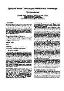
of search were proposed (40), with the aim of finding property violations sooner. Explicit Model Checking for CTL For CTL, we can use the observation that all the computational subtrees that start at a particular state are isomorphic. Thus, it is possible to mark each state with the set of subformulas of the checked property that hold for the subtree that starts with it (this property does not hold for LTL, because a state can appear on multiple suffixes of executions that start with it). This method can be performed recursively, starting by marking the states with propositional variables or their negation, depending on whether the state satisfies the propositional property. Boolean operators are applied in an obvious way, for example, if a node is marked with f and with g, then it will be marked with f ^ g. We will denote the set of nodes marked with a subformula f by Sf. For a set of states Q, we denote PredðQÞ ¼ fsj 9 s0 Rðs; s0 Þ ^ s0 2 Qg. Marking a node with EXf is also simple, just check whether this node has an edge to a node marked with f, i.e., Pred(Qf). The algorithm for marking nodes with E[fUg] and E[fRg] will be described below. Recall that we assume that all computations are infinite, which means that every state has a successor. procedure CheckEU; Q: ¼ ; Q 0 : ¼ Sg; while Q 6¼ Q 0 do Q: ¼ Q 0 ; Q 0 : ¼ Sg [ (Sf \ Pred(Q)); end while; mark states Q with E[f Ug]; procedure CheckER; Q: ¼ S; Q 0 : ¼ Sg; while Q 6¼ Q 0 do Q: ¼ Q 0 ; Q 0 : ¼ Sg \ (Sf [ Pred(Q)); end while; mark states Q with E [f Rg]; As an example of checking properties explicitly, consider the simple Kripke structure M in Fig. 1 on the alphabet S ¼ {a, b, c} and the CTL properties p1 ¼ E[cUb] and p2 ¼ EGa.

q0 c

q1 a, c

q3

q4

b

a

q2 a, b

Figure 1. An example of Kripke structure.

1910

MODEL CHECKING

We verify p1 using the procedure CheckEU. In M, Sb ¼ {q2, q3} and Sc ¼ {q0, q1}. In the initialization phase, Q ¼ ; and Q0 ¼ Sb ¼ {q2, q3}. Because Q 6¼ Q0 , the procedures execute the cycle body and Q becomes equal to Q0 (Q ¼ {q2, q3}) and Q0 is modified into Sb [ (Sc \ Pred({q2, q3})). Because q2 is reachable from q1 and q3 is reachable from q0, Q0 ¼ {q2, q3} [ ({q0, q1} \ {q0, q1}) ¼ {q0, q1, q2, q3}. Then the while condition is checked again and, because Q 6¼ Q0 , the cycle body is executed again. Q becomes equal to Q0 (Q ¼ {q0, q1, q2, q3}, and because the states in {q0, q1, q2, q3} are reachable from {q0, q1, q2, q3, q4}, Q ¼ {q2, q3} [ ({q0, q1, q2, q3}) ¼ {q0, q1, q2, q3}. Because Q0 is not changed, when the while condition is checked Q ¼ Q0 and the procedure terminates. To verify p2, it can be first rewritten as E[falseRa], hence, CheckER is used to verify the model against p2. Because Sfalse ¼ ; and Sa ¼ {q1, q2, q4}, Q and Q0 are initialized to {q0, q1, q2, q3, q4} and {q1, q2, q4}, respectively. Because Q 6¼ Q0 , the cycle body is executed and Q is changed into Q0 (Q ¼ {q1, q2, q4}), and Q0 is modified into Sa \ (Sfalse [ Pred({q1, q2, q4})). Because q1 is reachable from q0 and q4, q2 from q1 and q4 from q2 and q3, Q0 ¼ {q1, q2, q4} \ (; [ {q0, q1, q2, q3, q4}) ¼ {q1, q2, q4}. Now, Q0 is equal to Q, hence the procedure terminates, which marks the states in Q with p2. Explicit model checkers maintains a (hash) table of visited system states and a search stack. The size of these data structures often poses a severe limiting factor in explicit model checking. Several explicit specific techniques exist to prune the search considerably, as shown in the section ‘‘Dealing with complexity’’.

Many symbolic representations proposed in literature. 







Ordered Binary Decision Diagram (OBDD) (41) may sometimes have an extremely compact representation of Boolean formulas, as described in this section. Boolean Functional Vectors (BFV) (42) represent a bitlevel decomposition of the state-set, which is suitable for symbolic simulation. Affine equality or inequality relations (43) are defined among program variables; they are statically determined and used by the abstract interpretation (44). Boolean decision procedures, like Stalmarck’s Method (45) or the Davis and Putnam Procedure (46), are used by propositional decision procedures (SAT) (46) and have inspired symbolic model checking technique based on SAT procedures (47) as better explained in the section ‘‘Bounded Model checking’’.

OBDDs can be understood by first considering how Boolean formulas can be represented by binary decision trees. The internal nodes in the decision tree correspond to the variables of the formula. Edges and leaves are marked with true (1) and false (0). The value of the formula for a given assignment of values to the variables can be found by traversing the tree from root to a leaf. From each node, one progresses according to the edge labeled with the Boolean value assigned to the variable, which ends with a leaf that is marked with the Boolean value associated with the result of the Boolean function for the given assignment. This representation is not particularly compact, because it may store the same information repeatedly in different subtrees. OBDDs are derived from binary decision trees, but their structure is a directed acyclic graph instead of a tree. They are obtained by applying the following two steps: (1) combine any isomorphic subtree into a single tree and (2) eliminate any nodes whose two children are isomorphic. Therefore, redundant information in the structure is avoided by sharing common subtrees. The size of the resulting graph may be strongly dependent on the order of the variables. Figure 2(a) shows an example of binary decision tree and a truth table, in which each represents the function f ðX1; X2; X3Þ ¼ X1 X2 _ X1 X2 X3 _ X1 X2 X3. This binary decision tree can be transformed into the BDD

SYMBOLIC MODEL CHECKING In symbolic verification, the state space and the transition relation are not explicitly constructed but instead are symbolically represented. Often, systems have a structure with many repeated parts; this observation can be exploited so to reduce the space needed for representing the state transition graph considerably. More precisely, a symbolic verification algorithm deals with variables that denote sets of states, which are represented by Boolean functions instead of single states. It is clear that to put in practice the symbolic model checking technique, we need an efficient and automated method for representing and manipulating Boolean formulas.

X1 0 0 0 0 1 1 1 1

X1 1

0

X2 0

X2 1

X3 0

Figure 2. a) Binary decision tree and truth table of the function f ; b) BDD for the function f.

0

X3

1

X3

X2 0 0 1 1 0 0 1 1

X3 0 1 0 1 0 1 0 1

f 0 0 1 1 1 0 0 1

X1 1

0

X2

X2 0

0

X3

1

0

1

0

1

0

1

0

1

1

1

0

0

1

1

1

X3

0

0

1

1

0

(a)

0

1 (b)

X3

MODEL CHECKING

shown in Fig. 2(b) by maximally reducing it in according to the two rules before introduced. By using the original model checking algorithm with the new representation for transition relations, it becomes possible to verify systems that have more than 1020 states (48,49). Additional research results show that the state count can be more than 10120(50). Let M ¼ (S, R, L) be a finite Kripke structure, and let P(S) be the set of all subsets of S. A predicated transformer is a function that maps P(S) to P(S). Let t : PðSÞ ! PðSÞ be a function. Then ti ðZÞ denotes i repeated applications of t to Z 2 PðSÞ, where Z represents a set of states. It is recursively defined by t0 ðZÞ ¼ Z and tiþ1 ðZÞ ¼ tðti ðZÞÞ. A set S0  S is a fixpoint of a function t if tðS0 Þ ¼ S0 . A fixpoint S0  S of t is the least (or greatest) fixpoint, if it is the smallest (or greatest, respectively) under set containment. If t is monotonic, then it always has the least fixpoint, which is denoted by mZ tðZÞ, and the greatest fixpoint, which is denoted by nZ tðZÞ. We can identify each CTL formula f with the predicate on X that holds exactly for the set of states fsjM; sj ¼ f g. Then, each basic CTL operator may be characterized as the least or greatest fixpoint of an appropriate function t (51), where Z is a variable that represents a set of states from P(S).        

AF f1 ¼ mZ f1 _ AXZ EF f1 ¼ mZ f1 _ EXZ AG f1 ¼ nZ f1 ^ AXZ EG f1 ¼ nZ f1 ^ EXZ A½ f1 U f2 ¼ mZ f2 _ ð f1 ^ AXZÞ E½ f1 U f2 ¼ mZ f2 _ ð f1 ^ EXZÞ A½ f1 R f2 ¼ nZ f2 ^ ð f1 _ AXZÞ E½ f1 R f2 ¼ nZ f2 ^ ð f1 _ EXZÞ

Eliminating the AX operators by pushing negation inside, we can remain with only fixpoint formulas with the modal operators EX. The formula R(X, X0 ) represents symbolically the relationship between the variables X at the present state, and their corresponding primed copies X0 at the next state. One can then represent EXf as 9 X 0 ðRðX; X 0 Þ ^ f ðX 0 ÞÞ. Note that the existential quantification is over Boolean values, and thus as such it can be easily eliminated. Now, each fixpoint formula above is either the least or greatest fix-point over some Boolean transformation t. Depending on the case, one can then perform the model checking using the following two procedures for calculating fixpoints. Note the similarities of these procedures with the procedures in section ‘‘Explicit Model Checking for CTL.’’ Note also that the difference between these two procedures is only with the starting predicate: For calculating the least fixpoint, we start with true, whereas for calculating the greatest fixpoint, we start with false. procedure Check m(t); Z: ¼ false; Z0 : ¼ t(Z); while Z 6¼ Z0 do Z:=t(Z0 )

1911

end while; return(Z); procedure Check n(t); Z: ¼ true; Z0 : ¼ t(Z); while Z 6¼ Z0 do Z: ¼ t(Z0 ) end while; return(Z); DEALING WITH COMPLEXITY The state space explosion problem in model checking is a result of the exponential growth of the number of states of a system with the number of its concurrent components. In software model checking, even for sequential systems, one can already have a huge number of states; consider for example all the combinations of values of the program variables. The hardware on which such a program runs must allow at least that number of states as well. Thus, various strategies to deal with the state space explosion are essential to cope with its inherently high complexity. The techniques presented in this section are attempts to extend the size of the systems that can be verified. Partial-Order Reduction Partial-order reduction is a generic name for a collection of methods for reducing the state space needed for model checking asynchronous systems (52–54). Hence, it is mostly targeted for model checking concurrent systems. Originally, the idea behind partial-order reduction is inspired by the relationship between the partial order and the interleaving models of execution; in general, multiple linearizations exist for a single partial ordered execution. Such linearizations should not be distinguished by the specification (although many formalisms, such as LTL, can easily do so), as they describe essentially the same behavior. This concept gives motivation to base model checking merely on representatives, i.e., (at least) one linearization per partialorder execution. In practice, partial-order reduction methods do not achieve this goal, and could they be better called commutativity-based reductions. The main observation behind partial-order reduction is that concurrently executed actions a and b, which are applied to the same state s, result in the same state in either order of execution. That is, observing actions as deterministic state transformers, a(b(s)) ¼ b(a(s)) for each state s. In general, we say in this case that a and b are independent. In general, we assume a fixed independence relation between pairs of actions (but later, independence that is based also on the current state was suggested (55). This relationship can be calculated from the program, e.g., local actions of different processes are independent of each other.) An action a is invisible with respect to a set of propositions AP (practically, the propositions that appear in the checked property), if executing a does not change the propositions assigned to the state. That is, the propositions

1912

MODEL CHECKING

that hold in the state s and in a(s) are always the same. If a is invisible and independent of b, executing a from s and then b will result in the sequence s ! aðsÞ ! bðaðsÞÞ, where s and a(s) are labeled the same. Executing b first and then a will result in the sequence s ! bðsÞ ! aðbðsÞÞ, where b(s) and a(b(s)) have the same label. These two sequences are stuttering equivalent (56) (i.e., if collapsed the consecutive states with same labels in both the paths, they are identical). Conveniently, stuttering equivalent sequences cannot be distinguished by LTL formulas without the next time operator (56), and conversely, every LTL formula that cannot distinguish between stuttering equivalent sequences can be expressed using LTL without the next time operator (57). In this context, removing one state a(s) or b(s) would not affect the satisfiability of a stutter-closed specification. Removing just one such state would not make a big difference. However, when a lot of concurrency exists in the system, the overall reduction can be of several orders of magnitude. A popular partial-order reduction technique is called ample sets (58). It imposes the following principles in order to find a subset ample(s) of the actions that are executable or enabled in a state s. Then, one generates the reduced state graph for a system by expanding only the successors of s generated by the actions ample(s) rather than fully expanding s using all the actions enabled in s. Ample sets satisfy the following conditions: C1. After the state s, it is impossible to execute actions that are dependent on some actions from ample(s) before at least one action from ample(s) is executed. C2. If s is not fully expanded, then ample(s) includes only invisible actions. C3. Each cycle in the reduced graph of the model must contain at least one state that is fully expanded. Condition C1 can be achieved (e.g., by case analysis on the type of actions). For example, this condition is guaranteed when ample(s) consists of a single local action of some process (i.e., that changes only some of its local variables). Condition C2 is easy to check. Condition C3 can be implemented, for example, when using depth first search to generate the reduced state space as follows: when some action a taken from s generates a state a(s) that is already on the search stack, enforce that s is fully expanded. Many variations to this method are available, with subtle differences [e.g., stubborn sets (54) and persistent sets (52). Some other methods, such as sleep sets (59) and commutativity-based edge lean search (60), use a similar principle to exploit commutativity. Another family of partial-order reductions are based on unfolding (61) the partial order structure itself up to a certain size that is sufficient for model checking. Symmetry Systems under verification often present symmetries, which can be exploited to reduce the dimension of the model and, as a consequence, to improve the model-checking performance. Intuitively, two states can be considered symmetric if they can be interchanged without affecting

the system’s behavior. Roughly speaking, the symmetry relation among states can be used to build equivalence classes that substitute the states in the original Kripke structure (the transition relation is changed consequently), which strongly reduces the dimension of the model under verification. In the following, we introduce algebraic concepts needed to better understand the details on how symmetry reduction can be performed. A more detailed exposition can be found in Ref. 62. Given a set G and a binary operation , the pair hG, i2 is called group if (1)  is associative, (2) it has neutral element w.r.t. , and (3) 8 a 2 G, a admits inverse. H  G is a subgroup of G if it is a group w.r.t. . A permutation s on a finite mathematical object A is a bijection s : A ! A. The set of all the permutations of A, Sym A, which is also called full symmetric group, forms a group under functional composition. Its subgroups are called permutation groups. Given a Kripke structure M ¼ (S, R, L) and a permutation group G over S, a permutation s 2 G is called automorphism if and only if it preserves R [i.e., R,(s, s0 ) if and only if R(s(s),s(s0 ))]. G is called an automorphism group if and only if all the permutations in G are automorphism of M. Intuitively, an automorphism can be recognized as a symmetry of S, and the automorphism group is nothing but the set of all the automorphisms of S. The notion of automorphism group can be used to compute a set of symmetric states and, as a consequence, a quotient structure on it. Moreover an automorphism group G is called an invariance group for an atomic proposition p if and only if the set of states labeled by p is closed under the application of all the permutations of G. Indeed, given a Kripke structure M and an invariance group G for the set of the atomic proposition AP over which M is defined3, it is possible to construct a quotient structure MG ¼ (SG, RG, LG), which is defined as follows: 

 

SG ¼ fuðsÞjs 2 Sg, where uðsÞ ¼ ft j 9 s 2 GðsðsÞ ¼ tÞg is called the orbit of s; RG ¼ fðuðs1 Þ; uðs2 ÞÞjðs1 ; s2 Þ 2 Sg; LG ðuðsÞÞ ¼ Lðre pðuðsÞÞÞ, where rep(u(s)) is an arbitrary element of the orbit u(s).

It is possible to show that the quotient model is equivalent to the original one for model checking purposes; hence, it can be used instead of the original in the explicit state algorithm, as in Ref. 63, which saves considerable memory space. As example, consider a simple cache coherence protocol for a single bus multiprocessor system based on the Futurebus+ IEEE standard (64), which is verified in detail in Ref. 65. The system can be simply described as follows. Each processor contains a fixed number of cache lines, and they and the memory communicate through a single bus. At each bus cycle, the bus elects a master among the

2

Often the set G is used to denote the pair. The invariance allows one to build the labeling function of the quotient independently from the chosen representative. 3

MODEL CHECKING

processors, selects a cache line and a command, and puts them on the bus. The other processors and the memory react to the commands by changing their local context. The IEEE protocol under verification aims at guaranteeing the coherence of cache lines among different processors, which is exactly what has to be verified. The system behavior (i.e., the behavior of processors, memory and bus) can be described by a Kripke structure, in which the state of each processor is represented by the state of each its cache line and the state of bus interface. The bus is represented by the command on it, the active cache line, and other control signals. The system contains two symmetries: the processors and the cache lines. Let us concentrate only on processors symmetry in a system with N processes. If p1, j permutes the context of process 1 withQj, the symmetry group that uses processors symmetry is ¼ fp1; j j1  j  Ng and the set of representatives is composed by the states in which processor 1 is the master. The main limit of this method is that the problem of computing the orbits, which are necessary for the construction of the quotient structure, is at least as hard as the graph isomorphism problem, for which no known polynomial time algorithm is available. Hence, to lower the complexity of the implementation process, nonperfect ‘‘well-working’’ functions are used to compute the symmetries. These functions do not identify all symmetric states, but they never identify nonsymmetric states as symmetric. Symmetry can be exploited in with symbolic model checking (66, 67) and automata-based model checking (68). Moreover, Ref. 69 tries to exploit symmetry reduction also when the model exhibits little or no symmetry, which introduces guarded annotated quotient structures.

1913

5. If counterexample is a false negative, refine abstraction and repeat from step 2; 6. Otherwise, report concrete counterexample. In case of using linear specification (e.g., using LTL), the correctness criterion is defined in terms of language containments (the language of the specification includes the language of the system, as all the executions need to be ‘‘correct’’). For such a procedure to be useful, the relationship between the concrete system C and an abstract one A must satisfy that if Aw then C  w. In terms of languages, this result can be achieved if LðAÞ  LðCÞ. Thus, the abstraction, although being of smaller number of states, may include more executions, some of which are not allowed by the original model. Of course, we would like LðAÞ to be relatively close to LðCÞ to minimize the number of false negatives. Frequently, abstractions (71) are based on the notion of Galois connections (72). Let S be the set of concrete states, and Z be a set of abstract states. The pair (a, g) is a connection if:  

for each S  S, gðaðSÞÞ  S; and for each Z  Z, aðgðZÞÞ  Z.

The intuition is that moving from the concrete structure to an abstract one may reduce exactness, as multiple concrete subsets of states may be mapped to the same abstract one. Hence, when abstracting and then moving backward to the concrete states, we may obtain also these additional states. In fact, we can uniquely define g in a connection in terms of a and vice versa. That is: gðZÞ ¼

[

fS  S j aðSÞ  Zg

aðSÞ ¼

\

fZ  S j S  gðZÞg

Abstraction One can model a system at different ‘‘abstraction’’ levels. Often, a standard way of modeling exists, which can be obtained either automatically or manually following some well-accepted modeling principles. Then, one can consider a more abstract model with considerably fewer states. Although abstraction methods are very useful in making model checking more practical (i.e., checking considerably bigger systems), it is not guaranteed that a small abstract version will always exist. In a sense, it is not always the case that ‘‘in every system there is a smaller system that represents it well enough to be verified’’. Moreover, it can happen that some abstraction will work with some particular specification, whereas another one will work with the other. The abstraction needs to be related in a precise way to the original model so it will be useful as a practical replacement for verification. Abstraction can be performed using the following procedure: 1. Perform a first abstraction, using some standard technique (as shown below) (70); 2. Model checking the property against the abstract version; 3. If the verification passed, stop; 4. Otherwise, concretize the counterexample and compare it against the actual system;

The goal now is to define an abstract transition relation da  Z  Z in terms of a concrete transition relation dc  S  S using the connection. The relationship between these transition relations can be as follows: da ðs; s0 Þ when some concrete states t, t0 exist such that t0 2 gðfs0 gÞ and s 2 aðftgÞ. In other words, we simulate the abstract move from s to s0 by concretizing s, finding a corresponding concrete state t, following the transition relation d from t to t0 , and then abstracting t0 to find an abstract representative s0 . We can also perform this simulation backward rather than forward (from s0 to s through some t0 to t). This method is useful in particular when using symbolic model checking, where calculating the predecessors of states is simpler. One way of performing automatic abstraction symbolically is using the weakest precondition predicate transformer (73). For a given set of concrete states T, which satisfies exactly the predicate (formula) w, that is S ¼ fsjswg, we define the predicate transformer wpc(w) as a predicate that is satisfied exactly by the states S ¼ fsj 9 s0 ; dc ðs; s0 Þ ^ s0 wg. We start with a set of abstract values AV. These can be Boolean variables that correspond to the values of the predicates that appear in the model. It is important that the propositions of the checked properties can be interpreted over states from 2AV. Now for each formula w over the propositions AV, in particular any minterm w (conjunction of positive and negative occurrences from AV), we can

1914

MODEL CHECKING

define the set of abstract states from which we can reach w as those satisfying wpc(w). If wpc(w) calculates into an expression that involves other predicates than those in AV, then we may need to extend AV by including the latter predicates and repeat the abstraction. We may also apply a compositional abstraction (as example consider Ref. 74); because 2|AV| minterms exist with variables AV, we may calculate wpc(w) for w ¼ p or w ¼ :p, for each proposition p 2 AV. In case that such a weakest precondition is not based merely on values of AV, we may decide to allow both cases of true and false instead of refining AV. This method may add more false negatives, in which case additional refinement of the abstraction is needed.

FURTHER MODEL CHECKING APPROACHES Recently model checking approaches have been proposed for dealing with specific problems. In this section, we consider real-time model checking (presented in the next section) that aims at verifying systems with crucial timing constraints, probabilistic and stochastic model checking that gives also the answer to a probability of a failure, bounded model checking in that exploits the idea of checking if a property holds only on paths of predefined length instead on infinite paths, and compositional model checking that aims to deduce the correctness of a system (with respect to a specification) by model checking its subparts. Real-time Model Checking Among the proposed continuous time models (such as 75, 76), Timed Automata (TA) (77, 78) are frequently used. A TA is a finite state automaton enriched with a finite set of real-time clocks. Its transitions are instantaneous, whereas time elapses when the automaton is in a state (or location). Formally, if X is a finite set of clocks, then VX is the set of x the evaluations of X and GX  22 is the set of the assignments of X. Under each assignment g 2 GX , a set of the clocks are simultaneously reset to 0, whereas other clocks do not change. If n 2 VX and g 2 GX , then an evaluation n½g is such that, 8 x 2 X, n½g ðxÞ ¼ 0 if x 2 gðxÞ, and otherwise, n½g ðxÞ ¼ nðgðxÞÞ. We denote by n þ d, for d 2 Rþ , the passage of time from n by a quantity of d, which means that ðn þ dÞðxÞ ¼ nðxÞ þ d. A time constraint c is defined as c :¼ xcjx  x0 cjc ^ cj : c where  2 f ;
g. The constant c is in general a rational number; because the number of constants is finite, one may multiply them by the least-common multiple of their denominators to obtain integers. Henceforward, we shall, without loss of generality, assume that c is an integer. Given the set of constraints CX on X, a relation  is defined as follows:  

n xc if and only if nðxÞc; n x  x0 c if and only if n ðxÞ  n0 ðxÞc;

 

n c ^ c0 if and only if n c and n c0 ; n : c if and only if n 2 c.

A Timed Automata A ¼ (S, X, S, E, I) is a tuple, where S is a finite set of locations, X is a finite set of clocks, S is the set of labels, E is the transition relation, and I : S 7! CX is a set of state-invariants constraints for the states of the automaton. Each switch e ¼ (s, s, c, g, s0 ) in E has the following components: s and s0 are the initial and final locations, respectively; s 2 S is a label; c 2 CX is a guard (i.e., a time constraint); and g 2 GX is the assignment. Informally a switch represents a move from one location of the automaton to another. It is enabled only if the guard is satisfied by the clocks evaluation and, when it fires, the assignment is executed. The semantics of A can be explained through a transition system hQ; ! i, which is defined as follows: Q ¼ fðs; nÞ 2 S  VX jnIðsÞg; !  Q  ðS [ Rþ Þ  Q is defined by: Discrete transitions

ðs; s; c; g; s0 Þ 2 E nc; n½g Iðs0 Þ ðs; nÞ ! ðs0 ; n½g Þ þ

Timed transitions

d 2 Rþ 8 d0 2 R d0  d ) ðn þ d0 Þ 6¼ IðsÞ ðs; nÞ ! ðs; n þ dÞ

TAs can be checked through LTL model checking (79), CTL model checking (78), or performing reachability analysis (80) on the corresponding transition system. In all the cases, the problem is that, in general, the transition system is infinite. To overcome this problem, two main techniques are introduced. The first method consists in constructing a finite representation of TAs using clock regions instead of clock evaluations. A clock region represents a set of evaluations. Informally, if two states correspond to the same location and have clock evaluations with the same integer part and fractional part that respects the same order for all clocks, we say that the two states have a similar behavior. The integer part determines whether a guard or an invariant is satisfied or not, whereas the order of the fractional part fixes which clock will change its integer part first. A clock evaluation can grow arbitrarily. Let cx is the maximum value in the guards and invariants for the clock x, 8 x 2 X. Then, all the clock evaluations that exceed cx influence the behavior of the TA in the same way. If t 2 Rþ , let fr(t) the fractional part of t and b t c the integer part. The equivalence relation ffi on the possible clock assignments is defined as follows. Let n and n0 be two clock assignments. n ffi n0 if and only if the following three conditions are satisfied: 1. 8 x 2 X either nðxÞ
cx and n0 ðxÞ
cx or b nðxÞ c ¼ b v0 ðxÞ c 2. 8 x; y 2 X such that nðxÞ  cx and nðyÞ  cy ; frðnðxÞÞ  frðvðyÞÞ if and only if fr(n0 (x))fr(n0 (y)); 3. 8 x 2 X such that nðxÞ  cx ; frðvðxÞÞ ¼ 0, if and only if fr(n0 (x)) ¼ 0.

MODEL CHECKING

The equivalence classes induced by ffi are called region. [n] is a region that includes n. The number of regions induced by ffi is limited by |X|! 2|X| Px 2 X ð2cx þ 2Þ: Using the regions, a new transition system called region graph can be constructed: 





the states of the region graphs are (s, [n]), where s 2 S and [n] is a clock region; the initial state is (s0, [n]), where s0 2 S0 and n(x) ¼ 0, 8 x 2 X; ((s,[n]),a,(s0 , [n0 ])) is a transition of the region graph if and only if (s, w) ! (s0 , w0 ) for some w 2 [n] and w0 2 [n0 ].

The properties that, by construction, hold for the clock regions allow one to use the region graph instead of the original transition system for reachability analysis without loss of information. Another approach to finitize the state space of TA is to use zones. This construction is often more efficient than using the regions construction. The intuitive idea is to exploit guards and invariants in the TA. A zone is the convex hull solution of a set of clock constraints (i.e., it is the maximal set of clock assignments that satisfy these constraints). This concept can be efficiently represented in memory through difference bounded matrix (77). This matrix provides for each ordered pair of clocks x; y 2 X [ f0g, where 0 is a clock that is set constantly to 0, a constraint cx;y 2 R [ f1g, where either x  y < cx;y or x  y  cx;y . Although (infinitely) many representations may be available for the same convex hull that corresponds to the set of clock constraints, a unique normal representation always occurs. Normalization can be performed in cubic time. It can be shown that for TAs, only a finite number of zones are required. Furthermore, a transition relation can be defined between the zones (77).

Probabilistic and Stochastic Model Checking Probabilistic model checkers give an answer to the probability of a failure and also to its existence (81–83). They make use of techniques for calculating the probability of the occurrence of certain events during the execution of the system. Both the model and the properties to be checked contain the notion of probability; models encode the probability of making a transition between states instead of simply the existence of such a transition. The analysis normally calculates the actual probability of properties such as ‘‘What is the probability of this sequence of events?’’ Several probabilistic models have been proposed in the literature. The simplest is discrete-time Markov chains, in which the probability p(s, s0 ) of making a transition from one state s to another s0 is specified and the total probability P to reach s0 must be 1 (i.e., s0 pðs; s0 Þ ¼ 1). In continuoustime Markov chains, rðs; s0 Þ specifies the rates of making a transition from s to s0 with the interpretation that the probability of moving from s to s0 within tð 2 R > 0 Þ time 0 units is 1  erðs;s Þ t . The probabilistic specification is typically an extension of some temporal logics, such as PCTL (84), which is a prob-

1915

abilisticextensionofthe temporallogicCTL.Thislogicallows us to express the probability of the occurrence of events. Bounded Model Checking Bounded model checking exploits the idea of checking whether a property holds only on paths of a predefined length K, instead on infinite paths of the model. This method might seem at first sight a good way to find only the shallow errors in the systems. Instead, the method allows us to verify both liveness and safety properties and, in many cases, a right choice of K can guarantee the correctness of the whole system. Checking if an LTL property holds in a model corresponds to searching for a path that satisfies the negation of the property. Bounded model checking uses the observation, which was mentioned previously, that if a counterexample path for the checked property exists for a finite structure, then there is, in particular, such a path that is ultimately periodic. In the following, we will describe the method as firstly introduced in Ref. 47 and 85. Bounded model checking is composed by two main steps: 1. The model M, which is generally expressed as a Kripke structure, and the negation of an LTL property to be verified f are translated into propositional formulas ½½M

K and ½½ : f

K , respectively, 2. The formula ½½M

K ^ ½½f

K is given as input to a satisfiability (SAT) solver, such as Chaff (86) or MiniSat (87). If it is not satisfiable, then w holds in M, otherwise it does not. To transform M ¼ (S, I, R, L) into a propositional formula, consider a finite prefix S0, S1,. . ., sK of an infinite path p of M. A state of M can be represented using n ¼ d log2 ðjSjÞ e Boolean variables. Using this representation, ½½M

K is defined as the propositional formula that constrains a path of length K to be valid (i.e., to start from an initial state and respect the transition function). Hence, ½½M

K ¼ Iðs0 Þ ^ ^ K1 i¼0 Tðsi ; siþ1 Þ, where I(s0) is the characteristic function of the set of the initial states, and Tðsi ; siþ1 Þ is the characteristic function of the transition relation. The characteristic function of the transition relation is considered for all the steps of the path of length K. Notice that during the unwinding for each transition, a new set of state variables is introduced to represent the target of the transition. These variables are then used as source of the next transition in the path. When both the negation of the property and the model are translated in propositional formulas, a new formula given by the conjunction of the two is created. This last formula is given to a SAT solver to verify its satisfiability. SAT solving is known to be NP-complete (88). However, with modern heuristics, it is, in general, very efficient in practice. Many SAT solvers assume that the input problem is given in conjunctive normal form (CNF) (i.e., as conjunction of disjunctions). Rewriting a formula in CNF can lead to a formula exponentially bigger than the original. To avoid the exponential blow up, many methods were proposed, such as using a structure to preserve clause form transformation (89).

1916

MODEL CHECKING

Once checked with a SAT solver, if the formula is shown to besatisfiable(i.e., w does not hold in M), the providedexample works as the counterexample in classic model checking. When, instead, the formula is not satisfied, it may be because K is not big enough. Several methods deal with the problem of providing a good estimation of K (85, 90, 91). Compositional Model Checking Consider a system composed of many parallel processes. The idea of compositional model checking is to decompose the specification into properties that describe the behavior of small parts of the system, to check locally these properties, and to deduce from the local checks that the complete system satisfies the overall specification. By decomposing the verification in such a way we never have to compose all the processes, part of the state explosion problem is avoided. The main difficulty of this approach is that local properties are typically not preserved at the global level essentially because of mutual dependencies among the considered subparts of the system. Several approaches to compositional reasoning have been proposed recently: Partitioned transition relations (92) and lazy parallel composition (93) provide a way to compute the set of successors or predecessors of a state set without constructing the global system. The results are combined to give the set of states that compose the complete system. Assume-guarantee reasoning (94,95) is a technique that, considering a system composed of several compo-

nents, aims at verifying the system through the separate verification of the single components. More precisely, each single component cannot be considered isolate but behaving and interacting with its environment (i.e., the rest of the system). Actually, in assume guarantee, the environment is represented as a set of properties that it should satisfy to interact with the component correctly. These properties are called assumptions, which means that they are the assumptions that the component makes on the environment. If these assumptions are satisfied by the environment, then the component that behaves in this environment will satisfy other properties, which are called guarantees. By combining the set of assume/guarantee properties in an appropriate way, it is possible to demonstrate the correctness of the entire system without constructing the complete system. Several works propose suitable decompositions of the system [e.g., 96] and automatic generation of the assumptions [e.g. 97]. The most important problem of the compositional model checking techniques is the trade off between efficiency and automation. The problem with automatic techniques is that they typically rely on particular types of systems. MODEL CHECKING IN PRACTICE Various model checking tools have been proposed. In Table 1, we report some of them highlighting the type of model checker, the modeling and specification

Table 1. Model checking Tools Tool Bogor CBMC HyTech Java PathFinder Kronos MMC Moped MOPS Murphi NuSMV

PRISM ProB Rabbit Red SMV SPIN StEAM UPPAAL

Type of Model Checker

Modeling Language

Extensible and customizable, model checker Bounded model checking for C and C++ programs Symbolic model checker for hybrid systems Verification of executable Java bytecode programs Real-time systems verification (symbolic) Model checking .NET applications Model checker for pushdown systems Model checker for security properties Several versions are available BDD-based model checker SAT-based bounded model checker Probabilistic symbolic model checker Model checker for the B method Symbolic model checker for real-time systems Symbolic verification of timed/hybrid systems OBDD-based model checker Explicit LTL model checker Verification of native C++ programs Real-time systems verification

Specification Language

License

BIR

LTL

SAnToS License

C programs

Embedded

CBMC license

Hybrid automata

Embedded

Open Source

Java bytecode

Embedded

NASA license

Timed automata

TCTL

Free for academies

CIL bytecode programs

Embedded

Open source

Remopla

LTL

Open source

C programs

Finite State Automaton

Open source

Murphy description Like the language of SMV

LTL CTL + LTL

Open source LGPL v2.1

PRISM language

PCTL and CSL

GPL

XML encoding Timed automata

XML encoding Embedded

Open source Binaries

Timed automata

TCTL8

Red license

Network of automata Promela Machine-code Timed automata

CTL LTL Embedded CTL

Open source Open source Open source Free for academies

MODEL CHECKING

languages, and the kind of license under which the tool is released. After this general overview, we detail some frequently used model checking tools. In particular we focus on SPIN, which is a popular open-source model checker used by thousands of people worldwide; SMV, which is the first model checker based on BDDs; and Bogor, which allows the definition of new model checkers by extending and customizing it. Spin SPIN is an LTL model checker system (98) that may be used as an efficient verifier for many safety and liveness properties (e.g., invalid end states, unspecified receptions, flags incompleteness, race conditions). SPIN works on-the-fly, which means that it avoids the need to construct a global state graph, or a Kripke structure, as a prerequisite for the verification of any system properties. To optimize the verification runs, the tool exploits efficient partial order reduction techniques, and (optionally) BDD-like storage techniques. SPIN supports dynamically growing and shrinking numbers of processes. This permits to specify and analyze systems which evolve and change at run-time. Finally, SPIN supports random, interactive, and guided simulation. Promela (98) is the modeling language of SPIN and is a nondeterministic language, which is loosely based on Dijkstra’s guarded command language notation and borrows the notation for I/O operations from Hoare’s CSP language. Promela allows the modeling of concurrent systems that communicate via either message passing or shared variables. The key elements used in the language are processes, synchronous or asynchronous message channels, and variables. SMV The symbolic model verifier (SMV) (49) is the first OBDDbased model checker. The specification with respect to complex finite-state systems are satisfied is expressed in CTL. The system specification can be decomposed by means of modules. Modules can be instantiated multiple times, and each module can reference variables defined in other modules. Modules can be composed either synchronously (i.e., a single step in the composition corresponds to a single step in each component) or using interleaving (i.e., a single step of the composition corresponds to one step of exactly one component). The state transition in a model may be either deterministic or nondeterministic. The transition relation can be defined either explicitly (in terms of Boolean relations between the current state and the next state) or implicitly (as parallel assignments). Several extensions of SMV have been proposed in the last years and one of the most important is NuSMV (99) that combines BDD-based model checking with SAT-based model checking. Bogor Bogor (100) is an extensible software model checking framework that aims at supporting both general purpose and

1917

domain-specific software model checking. In particular, the extension and customization features of Bogor allow domain-experts to customize its input language and checking engine easily. The input language of Bogor, which is called BIR, simplifies the modeling of dynamic applications directly supports the dynamic creation of threads and objects, object inheritance, virtual methods, exceptions, garbage collection, and so on. The Bogor modeling language can be extended with new primitive types, expressions, and commands associated with a particular domain and a particular abstraction level. New algorithms (e.g., for state-space exploration, state storage, etc.) and new optimizations (e.g. heuristic search strategies, domain-specific scheduling, etc.) can be easily defined. ACKNOWLEDGMENTS Some of the authors are partially supported by ARTDECO (Adaptive infRasTruc-ture for DECentralized Organizations), an Italian FIRB (Fondo per gli Investimenti della Ricerca di Base) 2005 Project. BIBLIOGRAPHY 1. E. M. Clarke, and E. A. Emerson, Design and synthesis of synchronization skeletons using branching-time temporal logic, in Logic of Programs, New York: Springer-Verlag, 1982. 2. J. P. Queille, and J. Sifakis, Specification and verification of concurrent systems in CESAR, Proc. of the 5th Colloquium on International Symposium on Programming, 1982, pp. 337– 351. 3. E. M. Clarke, and J. M. Wing, Formal methods: State of the art and future directions, Technical Report CMU-CS-96-178, Carnegie Mellon University, 1996. 4. D. Peled, Software Reliability Methods, New York: Springer, 2001. 5. E. M. Clarke, O. Grumberg, and D. Peled, Model Checking, Cambridge, MA: MIT Press, 2001. 6. M. Sipser, Introduction to the Theory of Computation, Chapel Hill, NC: International Thomson Publishing, 1996. 7. A. Groce, and W. Visser, Heuristic model checking for java programs, Proc. of the 9th International SPIN Workshop on Model Checking of Software, 2002, pp. 242–245. 8. J. Esparza, Decidability of model checking for infinite-state concurrent systems, Acta Informatica 34 (2): 85–107, 1997. 9. J. Bormann, J. Lohse, M. Payer, and G. Venzl, Model checking in industrial hardware design, Proc. of the 32nd ACM/IEEE conference on Design automation (DAC 95), 1995, pp. 298–303. 10. S. Chandra, P. Godefroid, and C. Palm, Software model checking in practice: An industrial case study, Proc. of the 24th International Conference on Software Engineering (ICSE’02), 2002, pp. 431–441. 11. D. Peled, M. Y. Vardi, and M. Yannakakis, Black box checking, Proc. of the IFIP TC6 WG6.1 Joint International Conference on Formal Description Techniques for Distributed Systems and Communication Protocols (FORTE XII) and Protocol Specification, Testing and Verification (PSTV XIX), 1999, pp. 225–240. 12. E. A. Emerson, and J. Y. Halpern, ‘‘Sometimes’’ and ‘‘not never’’ revisited: On branching versus linear time temporal logic, J. ACM 33 (1): 151–178, 1986.

1918

MODEL CHECKING

13. K. L. McMillan, Using unfoldings to avoid the state explosion problem in the verification of asynchronous circuits, Proc. of the 4th International Workshop on Computer Aided Verification (CAV ’92), 1993, pp. 164–177. 14. J. Esparza, S. Romer, and W. Vogler, An improvement of mcmillan’s unfolding algorithm, Proc. of the 2nd International Conference on Tools and Algorithms for Construction and Analysis of Systems (TACAS ’96), 1996, pp. 87–106. 15. M. Kaufmann, M. Andrew, and C. Pixley, Design constraints in symbolic model checking, Proc. of the 10th International Conference on Computer Aided Verification (CAV ’98), 1998, pp. 477–487. 16. A. Prior, Time and Modality, London, UK: Oxford University Press, 1957. 17. A. Prior, Past, Present, and Future, London, UK: Oxford University Press, 1967. 18. E. M. Clarke, E. A. Emerson, and A. P. Sistla, Automatic verification of finite-state concurrent systems using temporal logic specifications, ACM Trans. Programming Lang. Syst., 8 (2): 244–263, 1986. 19. B. Alpern, and F. B. Schneider, Recognizing safety and liveness, Distributed Comput., 2 (3): 117–126, 1987. 20. Z. Manna, and A. Pnueli, Completing the temporal picture, Theoretical Comput. Sci. 83 (1): 91–130, 1991. 21. A. Pnueli, A temporal logic of concurrent programs, Theoretical Comput. Sci., 13: 45–60, 1981. 22. M. Ben-Ari, Z. Manna, and A. Pnueli, The temporal logic of branching time, Proc. of the 8th ACM SIGPLAN-SIGACT symposium on principles of programming languages (POPL’81), 1981, pp. 164–176. 23. J. R. Bu¨chi, On a decision method in restricted second order arithmetic, Proc. of the International Congress of Logic, Methodology and Philosophy of Science, 1960, pp. 1–11. 24. R. S. Streett, Propositional dynamic logic of looping and converse is elementarily decidable, Inf. Cont. 54 (1/2): 121– 141, 1982. 25. M. Y. Vardi, and P. Wolper, An automata theoretic approach to automatic program verification, Proc. of the 1st Symposium on Logic in Computer Science, 1986, pp. 332–344. 26. R. Gerth, D. Peled, M. Y. Vardi, and P. Wolper, Simple on-the-fly automatic verification of linear temporal logic, in Protocol Specification, Testing and Verification, New York: Springer, 1995. 27. P. Gastin, and D. Oddoux, Fast LTL to Bu¨chi automata translation, Proc. of the 13th International Conference on Computer Aided Verification (CAV’01), 2001, pp. 53–65. 28. P. Wolper, Temporal logic can be more expressive, Inf. Cont. 56 (1–2): 72–99, 1983. 29. W. Thomas, Automata on infinite objects, Handbook of Theoretical Computer Science (vol. B): Formal Models and Semantics, New York: Elsevier, 1990. 30. H. W. Kamp, Tense logic and the theory of linear order, PhD thesis, Los Angeles, California, UCLA, 1968. 31. D. Gabbay, A. Pnueli, S. Shelah, and J. Stavi, On the temporal analysis of fairness, Proc. of the 7th ACM SIGPLAN-SIGACT symposium on Principles of programming languages (POPL ’80), 1980, pp. 163–173. 32. D. Gabbay, The declarative past and imperative future: executable temporal logic for interactive systems, in Temporal Logic in Specification, New York: Springer-Verlag, 1987. 33. W. Thomas, Languages, automata, and logic, Handbook of Formal Languages, Vol. 3: Beyond Words, New York: Springer, 1997.

34. F. Somenzi, and R. Bloem, Efficient Bu¨chi automata from LTL formulae, Proc. of the 12th International Conference on Computer Aided Verification(CAV’00), 2000, pp. 248–263. 35. D. Giannakopoulou, and F. Lerda, From states to transitions: Improving translation of LTL formulae to Bu¨chi automata, Proc. of the 22nd IFIP WG 6.1 International Conference Houston on Formal Techniques for Networked and Distributed Systems (FORTE ’02), 2002, pp. 308–326. 36. R. Sebastiani, and S. Tonetta, ‘‘More deterministic’’ vs. ‘‘smaller’’ Bu¨chi automata for efficient LTL model checking, Proc. of the the 12th Advanced Research Working Conference on Correct Hardware Design and Verification Methods (CHARME 2003), 2003, pp. 126–140. 37. M. Y. Vardi, and P. Wolper, An automata-theoretic approach to automatic program verification (preliminary report), Proc. of Symposium on Logic in Computer Science (LICS’86), 1986, pp. 332–344. 38. C. Courcoubetis, M. Y. Vardi, P. Wolper, and M. Yannakakis, Memory-efficient algorithms for the verification of temporal properties, Formal Meth. Syst. Design1 (2–3): 275–288, 1992. 39. G. J. Holzmann, D. Peled, and M. Yannakakis, On nested depth first search, Proc. of 2nd SPIN Workshop. American Mathematical Society, 1996. 40. S. Edelkamp, S. Leue, and A. Lluch-Lafuente, Directed explicit-state model checking in the validation of communication protocols, Inter. J. Softwa. Tools Tech. Transf., 5 (2): 247–267, 2004. 41. R. E. Bryant, Graph-based algorithms for boolean function manipulation, IEEE Trans. Comput., C-35 (8): 677–691, 1986. 42. O. Coudert, C. Berthet, and J. C. Madre, Verification of sequential machines using boolean functional vectors, Proc. of the IFIP International Workshop on Applied Formal Methods for Correct VLSI Design, 1989, pp. 111– 128. 43. P. Cousot, and N. Halbwachs, Automatic discovery of linear restraints among variables of a program, Proc. of the 5th ACM SIGACT-SIGPLAN symposium on Principles of programming languages (POPL ’78), 1978, pp. 84–96. 44. P. Cousot, and R. Cousot, Static determination of dynamic properties of programs, Proc. of the 2nd International Symposium on Programming, 1976, pp. 106–130. 45. G. Sta˚lmarck, and M. Sa¨fiund, Modeling and verifying systems and software in propositional logic, Proc. of Safety of Computer Control Systems Conference (SAFECOMP’90), 1990, pp. 31–36. 46. M. Davis, and H. Putnam, A computing procedure for quantification theory, J. ACM 7 (3): 201–215, 1960. 47. A. Biere, A. Cimatti, E. Clarke, and Y. Zhu, Symbolic model checking without BDDs, Proc. of the 5th International Conference on Tools and Algorithms Construction and Analysis of system, 1999, pp. 193–207. 48. J. R. Burch, E. M. Clark, K. L. McMillan, D. L. Dill, and L. J. Hwang, Symbolic model checking: 1020 states and beyond, Inf. Computat., 98 (2): 142–170, 1990. 49. K. L. McMillan, Symbolic model checking: An approach to the state explosion problem, PhD thesis, Kluver Academic, 1993. 50. J. R. Burch, E. M. Clark, D. E. Long, K. L. McMillan, and D. L. Dill, Symbolic model checking for sequential circuit verification, IEEE Trans. Computer-Aided Design Int. Circuits13 (4): 401–424, 1994.

MODEL CHECKING 51. E. A. Emerson, and E. M. Clarke, Characterizing correctness properties of parallel programs using fixpoints, Proc. of the 7th Colloquium on Automata, Languages and Programming, 1980, pp. 169–181. 52. P. Godefroid, and D. Pirottin, Refining dependencies improves partial-order verification methods (extended abstract), Proc. of the 5th International Conference on Computer Aided Verification (CAV ’93), 1993, pp. 438–449. 53. D. Peled, Combining partial order reductions with on-the-fly model-checking, Proc. of the 6th International Conference on Computer Aided Verification (CAV ’94), 1994, 377–390. 54. A. Valmari, A stubborn attack on state explosion, Formal Meth. Syst. Design 1 (4): 297–322, 1992. 55. S. Katz, and D. Peled, Defining conditional independence using collapses, Theoretical Comput. Sci., 101 (2): 337–359, 1992. 56. L. Lamport, What good is temporal logic? Proc. of the IFIP 9th World Congress, 1983, pp. 657–668. 57. D. Peled, and T. Wilke, Stutter-invariant temporal properties are expressible without the next-time operator, Inf. Proc. Lett., 63 (5): 243–246, 1997. 58. D. Peled, All from one, one for all: On model checking using representatives, Proc. of the 5th International Conference on Computer Aided Verification (CAV ’93), 1993, pp. 409–423. 59. P. Godefroid, Using partial orders to improve automatic verification methods, Proc. of the 2nd International Workshop on Computer Aided Verification (CAV ’90), 1991, pp. 176–185. 60. D. Bosnacki, E. Elkind, B. Genest, and D. Peled, On commutativity based edge lean search, Proc. of the 34th Interantional Colloquium on Automata, Languages, and Programming (ICALP’97), 2007, pp. 158–170. 61. J. Esparza, and K. Heljanko, Unfoldings - A Partial-Order Approach to Model Checking, New York: Springer-Verlag, 2008. 62. J. J. Rotman, An Introduction to the Theory of Groups, New York: Springer-Verlag, 1995. 63. C. N. Ip, and D. L. Dill, Better verification through symmetry, in Computer Hardware Description Languages and their Applications, New York: Elsevier Science, 1993. 64. P. Robinson, IEEE Futurebus cache coherence protocol as a logic program, Microproc. Microsyst., 14 (8): 491–496, 1990. 65. E. M. Clarke, O. Grumberg, H. Hiraishi, S. Jha, D. E. Long, K. L. McMillan, and L. A. Ness, Verification of the Futurebus+ cache coherence protocol, Proc. of the 11th International Symposium on Computer Hardware Description Languages and their Applications, 1993, pp. 5–20. 66. E. A. Emerson, and R. J. Trefler, From asymmetry to full symmetry: New techniques for symmetry reduction in model checking, Proc. of the 10th IFIP WG 10.5 Advanced Research Working Conference on Correct Hardware Design and Verification Methods (CHARME ’99), 1999, pp. 142–156. 67. S. Barner, and O. Grumberg, Combining symmetry reduction and under-approximation for symbolic model checking, Proc. of the 14th International Conference on Computer Aided Verification (CAV ’02), 2002, pp. 93–106. 68. E. A. Emerson, and A. P. Sistla, Utilizing symmetry when model checking under fairness assumptions: an automatatheoretic approach, Proc. of the 7th International Conference on Computer Aided Verification (CAV’95), 1995, pp. 309– 324. 69. A. P. Sistla, and P. Godefroid, Symmetry and reduced symmetry in model checking, Proc. of the 13th International Conference on Computer Aided Verification (CAV ’01), 2001, pp. 91–103.

1919

70. E. M. Clarke, O. Grumberg, and D. E. Long, Model checking and abstraction, ACM Trans. Programming Lang. Sys., 16 (5): 1512–1542, 1994. 71. C. Loiseaux, S. Graf, J. Sifakis, A. Bouajjani, and S. Bensalem, Property preserving abstractions for the verification of concurrent systems, Formal Meth. Syst. Design, 6: 1–35, 1995. 72. M. Erne, J. Koslowski, A. Melton, and G. Strecker, A primer on galois connections, Proc. of the 1991 Summer Conference on General Topology and Applications in Honor of Mary Ellen Rudin and Her Work, 1993, pp. 103–125. 73. P. Cousot, Abstract interpretation: Theory and practice, Proc. of the 9th International SPIN Workshop on Model Checking of Software, 2002, pp. 2–5. 74. S. Chaki, J. Ouaknine, K. Yorav, and E. M. Clarke, Automated compositional abstraction refinement for concurrent c programs: A two-level approach, Elec. Notes Theoretical Comput. Sci. 89 (3), 2003. 75. T. A. Henzinger, X. Nicollin, J. Sifakis, and S. Yovine, Symbolic model checking for real-time systems, Proc. of the 7th Symposium of Logics in Computer Science (LICS ’92), 1992, pp. 394–406. 76. T. G. Rokicki, and C. J. Myers, Automatic verification of timed circuits, Proc. of the 6th International Conference on Computer-Aided Verification CAV’94, 1994, pp. 468–480. 77. D. Dill, Timing assumptions and verification of finite-state concurrent systems, Proc. of the International Workshop on Automatic Verification Methods for Finite State Systems, 1990, pp. 197–212. 78. R. Alur, C. Courcoubetis, and D. Dill, Model-checking for realtime systems, Proc. of the 5th Annual IEEE Symp. on Logic in Computer Science (LICS’90), 1990, pp. 414–425. 79. R. Alur, Techniques for automatic verification of real-time systems, PhD thesis, stanford, CA, Stanford University, 1992. 80. R. Alur, and D. Dill, Automata-theoretic verification of realtime systems, in Formal Methods for RealTime Computing. Trends in Software Series, New York: Wiley, 1996. 81. A. Aziz, V. Singhal, R. K. Brayton, and A. L. SangiovanniVincentelli, It usually works: The temporal logic of stochastic systems, Proc. of the 7th International Conference On Computer Aided Verification, 1995, pp. 155–165. 82. C. Baier, E. Clarke, V. Hartonas-Garmhausen, and M. Kwiatkowska, Symbolic model checking for probabilistic processes, Proc. of the 24th Interantional Colloquium on Automata, Languages, and Programming (ICALP’97), 1997. 83. C. Courcoubetis, and M. Yannakakis, The complexity of probabilistic verification, J. ACM42 (4): 857–907, 1994. 84. H. Hansson, and B. Jonsson, A logic for reasoning about time and probability, Formal Aspects Computing 6 (5): 512–535, 1994. 85. A. Biere, A. Cimatti, E. Clarke, O. Strichman, and Y. Zhu, Bounded model checking, Advances in Computers, Vol. 58, New York: Academic Press, 2003. 86. M. W. Moskewicz, C. F. Madigan, Y. Zhao, L. Zhang, and S. Malik, Chaff: Engineering an efficient SAT solver, Proc. of the 38th Design Automation Conference (DAC’01), 2001. 87. N. Ee´n, and N. So¨rensson, An extensible sat-solver, Proc. of International Conference on Theory and Applications of Satisfiability testing (SAT), 2003, pp. 502–518. 88. S. A. Cook, The complexity of theorem-proving procedures, Proc. of the 3rd annual ACM symposium on Theory of computing (STOC ’71), 1971, pp. 151–158.

1920

MODEL CHECKING

89. D. A. Plaisted and S. Greenbaum, A structure-preserving clause form translation, J. Symbolic Computat., 2 (3): 293– 304, 1986. 90. M. Sheeran, S. Singh, and G. Staalmarck, Checking safety properties using induction and a sat-solver, Proc. of the 3rd International Conference on Formal Methods in ComputerAided Design (FMCAD ’00), 2000, pp. 108–125. 91. O. Shtrichman, Pruning techniques for the SAT-based bounded model checking problem, Proc. of the 40th Conference on Design Automation, 2001, pp. 58–70. 92. J. R. Burch, E. M. Clarke, and D. E. Long, Symbolic model checking with partitioned transition relations, Proc. of the International Conference on Very Large Scale Integration (VLSI ’91), 1990. 93. S. V. Campos, A quantitative approach to the formal verification of realtime system, PhD thesis, SCS, Pittsburgh, PA: Carnegie Mellon University, 1996. 94. O. Grumberg, and D. Long, Model checking and modular verification, ACM Trans. Programming Lang. Syst., 16 (3): 843–871, 1994. 95. A. Pnueli, In transition for global to modular temporal reasoning about programs, Logics Models Concurrent Syst., 1984. 96. M. Caporuscio, P. Inverardi, and P. Pelliccione, Compositional verification of middleware-based software architecture descriptions, Proc. of the International Conference on Software Engineering (ICSE 2004), 2004. 97. D. Giannakopoulou, C. S. Pa˘sa˘reanu, and H. Barringer, Component verification with automatically generated assumptions, Auto. Softw. Eng., 12 (3): 297–320, 2005. 98. G. J. Holzmann, The SPIN Model Checker: Primer and Reference Manual, Boston, MA: Addison-Wesley, 2003. 99. A. Cimatti, E. M. Clarke, F. Giunchiglia, and M. Roveri, NUSMV: A new symbolic model verifier, Proc. of the 11th International Conference on Computer Aided Verification (CAV), 1999, pp. 495–499. 100. M. Robby, B. Dwyer, and J. Hatcliff, Bogor: An extensible and highly-modular software model checking framework, SIGSOFT Softw. Eng. Notes 28 (5): 267–276, 2003.

DORON PELED The University of Warwick Coventry, United Kingdom Bar Ilan University Ramat Gat, Israel

PATRIZIO PELLICCIONE Universita´ dell’Aquila L’Aquila, Italy

PAOLA SPOLETINI Universita´, dell’Insurbia Como, Italy