Symbolic Model Checking of Hybrid Systems ... - Computer Science

Symbolic Model Checking of Hybrid Systems using Template Polyhedra Sriram Sankaranarayanan1, Thao Dang2 and Franjo Ivanˇci´c1 1. NEC Laboratories America, Princeton, NJ, USA. 2. Verimag, Grenoble, France. {srirams,ivancic}@nec-labs.com,[email protected]

Abstract. We propose techniques for the verification of hybrid systems using template polyhedra, i.e., polyhedra whose inequalities have fixed expressions but with varying constant terms. Given a hybrid system description and a set of template linear expressions as inputs, our technique constructs over-approximations of the reachable states using template polyhedra. Therefore, operations used in symbolic model checking such as intersection, union and post-condition across discrete transitions over template polyhedra can be computed efficiently using template polyhedra without requiring expensive vertex enumeration. Additionally, the verification of hybrid systems requires techniques to handle the continuous dynamics inside discrete modes. We propose a new flowpipe construction algorithm using template polyhedra. Our technique uses higher-order Taylor series expansion to approximate the time trajectories. The terms occurring in the Taylor series expansion are bounded using repeated optimization queries. The location invariant is used to enclose the remainder term of the Taylor series, and thus truncate the expansion. Finally, we have implemented our technique as a part of the tool TimePass for the analysis of affine hybrid automata.

1

Introduction

Symbolic model checking of infinite state systems requires a systematic representation for handling infinite sets of states. Commonly used representations include difference matrices, integer/rational polyhedra, Presburger arithmetic, polynomials, nonlinear arithmetic and so on. Expressive representations can better approximate the underlying sets. However, the basic operations required for symbolic execution such as intersection, image (post-condition) and so on are harder to compute on such representations. Convex polyhedra over reals (rationals) are a natural representation of sets of states for the verification of hybrid systems [15, 30, 2, 10–12]. However, basic algorithms required to manipulate polyhedra require worst-case exponential complexity. This fact has limited the practical usefulness of symbolic model checking tools based on polyhedra. Therefore, restricted forms of polyhedra such as orthogonal polyhedra [3] and zonotopes [11] are used to analyze larger systems at a level of precision that is useful for proving some properties of interest. Other

techniques, such as predicate abstraction, use Boolean combinations of a fixed set of predicates p1 , . . . , pm , to represent sets of states [1, 16]. Such techniques enable the refinement of the representation based on counterexamples. In this paper, we propose template polyhedra as a representation of sets of states. Given a set of template expressions e1 , . . . , em , we obtain V a family of template polyhedra, each of which is represented by the constraints i ei ≤ ci [29]. As with predicate abstraction, our approach assumes that the template expressions are provided as an input to the reachability problem. We then use the family of polyhedra defined by the given template expressions as our representation for sets of states. The advantage of restricting our representation to a family of template polyhedra is that operations such as join, meet, discrete post-condition and time elapse can be performed efficiently, without requiring expensive vertex enumeration. Furthermore, our initial experience suggests that commonly used domains in software analysis such as intervals and octagons provide a good initial set of templates. This set can be further refined using simple heuristics for deriving additional expressions. In order to analyze hybrid systems, we additionally require techniques to over-approximate the continuous dynamics at some location. This paper proposes a sound flowpipe construction technique based on a Taylor series approximation. Our approach works by solving numerous linear programs. The solutions to these linear programs correspond to bounds on the terms involved in the Taylor series expansion. The expansion itself is bounded by enclosing the remainder term using the location invariant. The flowpipe construction results in a series of template polyhedra whose disjunctions over-approximate the time trajectories. Finally, we have implemented our methods in our prototype tool TimePass for verifying safety properties of affine hybrid systems. We use our tool to analyze many widely studied benchmark systems and report vastly improved performance on them. Related Work Hybrid systems verification is a challenge even for small systems. Numerous approaches have been used in the past to solve reachability problems: the HyTech tool due to Henzinger et al. uses polyhedra to verify rectangular hybrid systems [15]. More complex dynamics are handled using approximations. Kurzhanski and Variaya construct ellipsoidal approximations [17]; Mitchell et al. use level-set methods [20]; the d/dt system uses orthogonal polyhedra and face lifting [2]; Piazza et al. [22] propose approximations using constraint solving based on quantifier elimination over the reals along with Taylor series expansions to handle the continuous dynamics. Lanotte & Tini [18] present approximations based on Taylor series that can be made as accurate as possible, approaching the actual trajectories in the limit. Girard uses zonotopes to construct flowpipes [11]. The PHAVer tool due to Frehse extends the HyTech approach by repeatedly subdividing the invariant region and approximating the dynamics inside each subdivision by piece-wise constant dynamics [10]. Tiwari [31] presents interesting techniques for proving

safety by symbolically integrating the dynamics of the system. Symbolic techniques for proving unreachability without the use of an explicit flowpipe approximation [28, 32, 26, 23]. These techniques can handle interesting nonlinear systems beyond the reach of many related techniques. The problem of flowpipe construction for template polyhedra has been studied previously by Chutinan & Krogh [5]. Their technique has been implemented as a part of the tool CheckMate [30]. Whereas the CheckMate approach solves global non convex optimization problems using gradient descent, our approach solves simple convex optimization problems to bound the coefficients of the Taylor series expansion. Furthermore, our technique can be extended to some nonlinear systems to construct ellipsoidal and polynomial flowpipes. The CheckMate technique simply yields a harder nonconvex optimization problem for these cases. On the other hand, our approach loses in precision due to its approximation of functions by Taylor polynomials; CheckMate, however, is more robust in this regard. Template polyhedra are commonly used in static analysis of programs for computing invariants. Range analysis can be regarded as template polyhedra over expressions of the form ±x [7] . Similarly, Vthe octagon domain due to Min´e [19] uses template polyhedron of the form xi − xj ≤ c. General template polyhedra were used as an abstract domain to represent sets of states by Sankaranarayanan et al. [29].

2

Preliminaries

Let R denote the set of reals, and R+ = R ∪ {±∞}. A first order assertion ϕ[x1 , . . . , xn ], over the theory of reals, represents a set [[ϕ]] ⊆ Rn . A column vector, denoted hx1 , . . . , xn i, is represented succinctly as x. Capital letters A, B, C and X, Y, Z denote matrices; Ai denotes the ith row of a matrix A. A linear function f (x) is the inner product of vectors cT x. Similarly, an affine function is represented as cT x + d. Polyhedra. A polyhedron is a conjunction of finitely many linear inequalities V e ≤ c, represented succinctly as Ax ≤ b, where A is a m × n matrix, b is a i i m × 1 column vector and ≤ is interpreted entry-wise. A linear program(LP) P : max. cT x subject to Ax ≤ b seeks to optimize a linear objective cT x over the convex polyhedron [[Ax ≤ b]]. If [[Ax ≤ b]] is nonempty and bounded then the optimal solution always exists. LPs are solved using techniques such as Simplex [8] and interior point techniques [4]. The former technique is polynomial time for most instances, whereas the latter can solve LPs in polynomial time. Vector Fields and Lie Derivatives. A vector field D over Rn associates each point x ∈ Rn with a derivative vector D(x) ∈ Rn . Given a system of differential equations of the form x˙i = fi (x1 , . . . , xn ), we associate a vector field D(x) = hf1 (x), . . . , fn (x)i. A vector field is affine if the functions f1 , . . . , fn are all affine in x. For instance, the vector field D0 (x, y) : hx + y, x − 2y − 3i is affine.

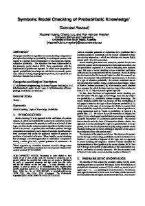
Let D(x) = hf1 (x), . . . , fn (x)i be a vector field over Rn . The Lie derivative of a and differentiable function h : Rn 7→ R is LD (f ) = (∇h)·D(x) = Pn continuous ∂h · f (x). The Lie derivative of the function x + 2y − 2 over the vector i i=1 ∂xi field D0 (x, y) shown above is given by LD0 (x + 2y − 2) = 1 · (x + y) + 2 · (x − 2y − 3) = 3x − 3y − 6 . Hybrid Systems. To model hybrid systems we use hybrid automata [14]. Definition 1 (Hybrid Automaton). A hybrid automaton Ψ : hn, L, T , Θ, D, I, ℓ0 i consists of the following components: – n is the number of continuous variables. These variables are denoted by the set V = {x1 , . . . , xn }. – L, a finite set of locations; ℓ0 ∈ L is the initial location; – T , a set of (discrete) transitions. Each transition τ : hℓ1 → ℓ2 , ρτ i ∈ T consists of a move from ℓ1 ∈ L to ℓ2 ∈ L, and an assertion ρτ over V ∪ V ′ , representing the transition relation; – Assertion Θ, specifying the initial values of the continuous variables; – D, mapping each ℓ ∈ L to a vector field D(ℓ), specifying the continuous evolution in location ℓ; – I, mapping each ℓ ∈ L to a location invariant, I(ℓ). A computation of a hybrid automaton is an infinite sequence of states hl, xi ∈ L × Rn of the form hl0 , x0 i, hl1 , x1 i, hl2 , x2 i, . . ., such that initially l0 = ℓ0 and x0 ∈ [[Θ]]; and for each consecutive state pair hli , xi i, hli+1 , xi+1 i, satisfies one of the consecution conditions: Discrete Consecution: there exists a transition τ : hℓ1 , ℓ2 , ρτ i ∈ T such that li = ℓ1 , li+1 = ℓ2 , and hxi , xi+1 i |= ρτ , or Continuous Consecution: li = li+1 = ℓ, and there exists a time interval [0, δ), δ > 0, and a time trajectory τ : [0, δ] 7→ Rn , such that τ evolves from xi to xi+1 according to the vector field at location ℓ, while satisfying the location condition I(ℓ). Formally, 1. τ (0) = x1 , τ (δ) = x2 , and (∀ t ∈ [0, δ]), τ (t) ∈ [[I(ℓ)]], 2. (∀t ∈ [0, δ)), dτ dt = D(ℓ)|x=τ (t) . Definition 2 (Affine Hybrid Automaton). A hybrid automaton Ψ is affine if the initial condition, location invariants and transition relations are all represented by a conjunction of linear inequalities; and furthermore, the dynamics at each location D(ℓ) is an affine vector field. The rest of the paper focuses solely on affine systems. However, our results also extend to the non-affine case. Example 1. Affine hybrid systems are used to represent a variety of useful systems. Consider the oscillator circuit shown in Figure 1(a). The circuit consists of a capacitor that may be charged or discharged using a voltage triggered switch S that is controlled by the voltage across the capacitor Vc . The corresponding

R

S

C

5V

(a)

Loc. C 1 V˙c = RC (5 − Vc ) t˙ = 1

Vc ≥ 4.5 t := 0

Vc ≤ 0.5

Loc. D c V˙c = −V RC t˙ = 1

(b)

Fig. 1. An oscillator circuit (left) and its affine hybrid automaton model.

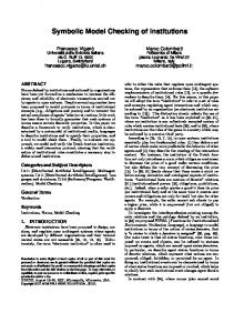
affine hybrid automaton H has two modes C and D corresponding to the charging and discharging; and two variables Vc modeling the voltage of the capacitor and t modeling time. Switching between each mode takes place when the capacitor has charged (or discharged) to 90% (10%) of its final charge. We assume the mode invariants I(C) : 0 ≤ Vc ≤ 4.5 and I(D) : 0.5 ≤ Vc ≤ 5. The post-condition and time elapse operations are the two fundamental primitives for over-approximating the reachable sets of a given hybrid automaton. Given an assertion ϕ over the continuous variables, its post-condition across a transition τ : hℓ, m, ρi is given by post(ϕ, τ )[y] : (∃ x) (ϕ(x) ∧ ρ(x, y)). The post-condition of a polyhedron is also polyhedral. It is computed using intersection and existential quantification. Similarly, given an assertion ϕ, the set of possible time trajectories inside a location ℓ with invariant I(ℓ) and dynamics D(ℓ) is represented by its time elapse ψ : timeElapse(ϕ, hD, Ii). However, for affine hybrid systems, the time elapse of a polyhedron need not be a polyhedron. Therefore, the time elapse operator is hard to compute and represent exactly. It is over-approximated by the union of a set of polyhedra. Such an approximation is called a flowpipe approximation. Using post-conditions and time elapse operators as primitives, we can prove unreachability of unsafe states using a standard forward propagation algorithm. Such an algorithm is at the core of almost all safety verification tools for hybrid systems [15, 2, 30, 10] Template Polyhedra. The goal of this paper is to implement symbolic model checking on hybrid systems using template polyhedra. We now present the basic facts behind template polyhedra, providing algorithms for checking inclusion, intersection, union and post-condition. Additional details and proofs are available from our previous work [29]. A template is a set H = {h1 (x), . . . , hm (x)} of linear expressions over x. We represent a template as an m × n matrix H, s.t. each row Hi corresponds to the linear expression hi . Given a template, a family of V template polyhedra may be obtained by considering conjunctions of the form i hi (x) ≤ ci . Each polyhedron in the family may be obtained by choosing the constant coefficients c1 , . . . , cm .

hH, (1, 1, 1, 1, ∞, ∞)i (a)

hH, (1, ∞, 1, 4, 3, 3)i hH, (1, ∞, ∞, ∞, 3, ∞)i (b)

(c)

no representation (d)

Fig. 2. Polyhedra (a), (b) and (c) are template instances for the template H shown in Example 2, whereas (d) is not.

Definition 3 (Template Polyhedron). A template polyhedron over a template H is a polyhedron of the form Hx ≤ c, wherein c ∈ Rm + . Such a polyhedron will be represented as hH, ci. Example 2. Consider the template H = {x, −x, y, −y, y − x, x − y}. The unit square −1 ≤ x ≤ 1 ∧ −1 ≤ y ≤ 1 may be represented by the template polyhedron hH, (1, 1, 1, 1, ∞, ∞)i. Figure 2 shows three polyhedra that are instances, and one that is not. Let c1 ≤ c2 signify that for each row i ∈ [1, |c1 |], c1 i ≤ c2 i . Lemma 1. If c1 ≤ c2 then hH, c1 i ⊆ hH, c2 i. However, the converse need not hold. Example 3. The set C : x = 0 ∧ y = 0 may be represented using the template H = {x, −x, y, −y, x + y} using the instances vectors c : h0, 0, 0, 0, 0i, c1 : h0, 0, 0, 0, 100i, c2 : h−10, 0, 0, 0, 0i, and c3 : h0, −100, 0, 0, 0i. In each case hH, ci i ⊆ hH, ci. However ci 6≤ c. Intuitively, “fixing” any four of the rows to 0 renders the remaining constraint row redundant. Consider a region C ⊆ Rn and template H. There exists a smallest template polyhedron hH, ci, with the least instance vector c, that over-approximates C, denoted c = αH (C). Furthermore, for any template polyhedra hH, di that overapproximates C, c ≤ d. Each component ci of αH (C) may be computed using the optimization problem ci : max. hi (x) s.t. x ∈ C. Note that if C is a polyhedron, then its best over-approximation according to a template H is obtained by solving |H| linear programs. Lemma 2. For any closed set C ⊆ Rn , the polyhedron Hx ≤ αH (c) is the smallest template polyhedron that includes C. Example 4. Let H = {x, −x, y, −y} be a template. Consider the set C : (x2 + y 2 ≤ 1) of all points inside the unit circle. The smallest template polyhedron

containing C is the unit square that may be represented with the instance vector h1, 1, 1, 1i. Additionally, if the expressions x + y, x − y, −x − y, x + y are added to the set H, the smallest template polyhedron representing C is the octagon inscribed around the circle. It is algorithmically desirable to have a unique representation of each set by a template polyhedron. Given a template polyhedron hH, ci, its canonical form is given by canH (c) = αH (Hx ≤ c). An instance vector is canonical iff c = canH (c). Lemma 3. (a) hH, ci ≡ hH, di iff canH (c) = canH (d), and (b) hH, ci ⊂ hH, di iff canH (c) < canH (d). Thus, canonicity provides an unique representation of template polyhedra. Any representation can be converted into a canonical representation in polynomial time using optimization problems. The union of hH, c1 i and hH, c2 i (written c1 ⊔c2 ) is defined as c = max(c1 , c2 ), where max denotes the entry-wise minimum. Similarly, intersection of two polyhedra c1 , c2 is represented by c = min(c1 , c2 ). Given a template polyhedron P0 : hJ, ci, and a discrete transition relation τ , we wish to compute the smallest template polyhedron P1 : hH, di that overapproximates the post-condition post(P0 , τ ). Note that the templates J and H need not be identical. The post-condition d : postH (hJ, ci , τ ) is computed by posing an optimization query for each di : max. Hi y subj. to Jx ≤ c ∧ ρτ (x, y). The resulting d is always guaranteed to be canonical. Lemma 4. The polyhedron postH (P0 , τ ) is the smallest template polyhedron containing post(P0 , τ ). In program analysis, template polyhedra with a fixed set of template have been used previously. For instance, given variables x1 , . . . , xn , intervals are obtained as template polyhedra over the set HI = {x1 , −x1 , x2 , . . . , xn , −xn } [7]. Similarly, the octagon domain is obtained by considering the template expressions HO = HI ∪ {±xi ± xj |1 ≤ i < j ≤ n} [19]. Other domains based on template polyhedra include the octahedron domain consisting of all linear expressions involving the variables x1 , . . . , xn with unit coefficients [6].

3

Flowpipe Construction

We now consider flowpipe construction techniques to over-approximate the time trajectories of affine differential equations. An instance of flowpipe construction problem: hH, c0 , inv, D, δi consists of the template H, an initial region hH, c0 i, the location invariant hH, invi and an affine vector field D representing the dynamics and a time step δ ≥ 0. We assume that hH, invi and hH, c0 i are nonempty and bounded polyhedra. Example 5. Consider the oscillator circuit model from Example 1. An instance consists of a template H = {v, −v, t, −t, v − t, t − v}, initial condition v ∈ [0, 0.1], t = 0 and location invariant v ∈ [0, 5], t ∈ [0, 100].

Let F(t) denote the set of states reachable, starting from hH, c0 i, at some time instant t ≥ 0. Similarly, F[t, t + δ) denotes the set of reachable states for the time interval [t, t + δ). Formally, we wish to construct a series of flowpipe segments hH, d0 i , hH, d1 i , hH, d2 i , . . . , hH, dN i , . . . such that each segment dj over-approximates F[jδ, (j + 1)δ). There are two parts to our technique: Flowpipe Approximation: Approximate F[0, δ) given hH, c0 i. Set Integration: Given an approximation F[iδ, (i + 1)δ), approximate the next segment F[(i + 1)δ, (i + 2)δ). Together, they may be used to incrementally construct the entire flowpipe. Set Integration. By convention, the j th order Lie derivative of a function f is written f (j) . Let f : cT x be a linear function. By convention, we denote its j th order derivative as c(j) x. Definition 4 (Taylor Series). Let h be a continuous function and differentiable at least to order m + 1. It follows that h(t) = h(0) + h(1) (0)t + h(2) (0)

t2 tm tm+1 + · · · + h(m) (0) + h(m+1) (θ) , 2! m! (m + 1)!

where θ ∈ [0, t). The last term of the series is known as the remainder. Let Sk : hH, dk i be an over-approximation of F[kδ, (k+1)δ). We wish to compute an approximation Sk+1 for the time interval [(k + 1)δ, (k + 2)δ). In other words, we require an upper bound for the value of each template row Hi x. Let x(t) be the state at time instant t. Using a Taylor series expansion, we get: Hi x(t + δ) = Hi x(t) + · · · +

δ m+1 δ m (m) (m+1) x(t + θ) , Hi x(t) + H m! (m + 1)! i

(1)

where 0 ≤ θ < δ. Note that the first m terms are functions of x(t), whereas the remainder term, is a function of x(t + θ). The exact value of θ is not known and is conservatively treated as a nondeterministic input. In other words, we may write Hi x(t + δ) as a sum of two expressions Hi x(t + δ) = gi T x(t) + ri T x(t + θ), wherein gi represents the sum of the first m terms of the Taylor series and ri represents the remainder term. Assuming t ∈ [jδ, (j + 1)δ), we have x(t) ∈ Sk . Therefore, an upper bound on gi is obtained by solving the following LP: gimax = max. gi T x subj.to. x ∈ Sk

(2)

Similarly, even though the remainder term cannot be evaluated with certainty, we know that x(t + θ) ∈ hH, invi. A bound on ri x(t + δ) is, therefore, obtained by solving the optimization problem rimax = max. ri T y subj.to y ∈ hH, invi

(3)

The overall bound on Hi x(t + δ) is gimax + rimax . Finally, the over-approximation Sk+1 is obtained by computing gimax + rimax for each template row i ∈ [1, |H|]. Note that in the optimization problem above, the time step δ is an user-input (m) constant, each Lie-derivative gi is affine and Sk is a template polyhedron. As a result, the optimization problems for affine vector fields are linear programs. Example 6. Following Example 5, consider a flowpipe segment v ∈ [0, 0.2] ∧ t ∈ ˙ [0, 0.1] by δ = 0.1, according to the differential equation v˙ = 5−v 2 , t = 1. The first row of the template is H1 : v. The first 6 Lie derivatives of H1 are tabulated below: 0 1 2 3 4 5 6 −5+v 5−v −5+v 5−v −5+v v 5−v 2 4 8 16 32 64 Following, Eq. 1, we use exact arithmetic to obtain 2

6

−5+v(θ) δ −5+v δ 5−v 5 v(t + δ) = v + 5−v 2 δ+ 4 2! + · · · + 32 δ 5! + 64 6! ∼ 0.951229424479167v(0) + 0.24385288020833 + 0.131 × 10−7 v(θ) {z } | {z } | r0

g0

g0max

Now observing that v(0) ∈ [0, 0.2], we obtain = 0.4341 (upto 4 decimal places). Similarly, using the location invariant v(θ) ∈ [0, 5], we obtain r0max = 0.131 × 10−8 × 5. As a result, we obtain a bound v(t + 0.1) ≤ 0.4341 (upto 4 decimal digits). Repeating this process for every template row gives us the required flowpipe approximation for the segment [0.1, 0.2). Flowpipe Approximation We now seek an approximation hH, d0 i for F[0, δ). Therefore, for each template row Hi , we wish to bound the function Hi x as an univariate polynomial of degree m + 1 over the time interval [0, δ). Let ai,j , 0 ≤ j ≤ m be the result of the optimization ai,j = max

(j)

Hi

(x) j!

subj.to. x ∈ hH, c0 i and ai,m+1 =

(m+1) Hi (y)

max m+1! subj.to. y ∈ hH, invi . Each optimization problem is an LP and can be solved efficiently. Consider Pm the polynomial pi (t) = j=0 aij tj + ai,m+1 tm+1 . Lemma 5. For t ≥ 0 and x ∈ hH, c0 i, Hi x(t) ≤ pi (t). (1)

Hi x(t) = Hi x(0) + tHi x(0) + · · · + tm

(m)

Hi

(x(0)) m!

+ tm+1

≤ ai0 + ai1 t + · · · + aim tm + ai,m+1 tm+1 ∵ ≤ pi (t)

(m+1)

Hi

(x(θ)) (m+1)!

(j)

Hi

x(0) j!

≤ aij and t ≥ 0

The required bound for the function Hi x for the time interval t ∈ [0, δ) may now be approximated by maximizing the univariate polynomial pi (t) over the interval [0, δ). The maximum value of an univariate polynomial p in a time interval [T1 , T2 ] may be computed by evaluating the polynomial at the end points T1 , T2 and the roots (if any) of its derivative p′ lying in that interval. The maxima in the interval is guaranteed to be achieved at one of these points.

4

4

3

3

V

5

V

5

2

2

1

1

0

0

2

4

6

8

10

12

14

0

0

10

20

30

t

t

(a)

(b)

40

50

Fig. 3. Flowpipes for Example 1: (a) one complete charge/discharge cycle and (b) the time interval [0, 49].

Example 7. Consider the problem instance shown in Example 5. We wish to compute an over-approximation of F[0, 0.1) given v(0) ∈ [0, 0.1] and t(0) = 0. We consider a bound H1 : v over t ∈ [0, 0.1). Example 6 shows the lie derivatives. The following table shows the bounds a1 , . . . , a6 corresponding to the initial condition and invariant regions (accurate to 4 decimal places). 0 1 2 3 4 5 6 0.1 2.5 −0.6125 0.1058 −0.01276 0.0013 −0.00106 As a result, we have that v(t) ≤ −0.00106t6 + 0.0013t5 − 0.01276t4 + · · · + 0.1 for all t ∈ [0, 0.1). This polynomial is increasing in this range and has its maximum value at t = 0.1. This yields a bound v ≤ 0.3439 for the segment F[0, 0.1). Similarly, we can compute bounds for all the rows in the template. Thus, given an instance of the flowpipe problem, we compute an initial flowpipe segment hH, d0 i ⊇ F[0, δ) by computing univariate polynomials, one per template row, that upper bound the Taylor series and in turn finding the maxima of these polynomials. This initial flowpipe segment is then advanced by using set integration. Following this scheme, Fig. 3 shows the flowpipe constructed for the instance in Example 5. Let d0 , . . . , dN be the results of the flowpipe construction on a given instance. WN Theorem 1. The disjunction i=0 hH, di i contains all the time trajectories starting from hH, c0 i and evolving according to D inside hH, invi. Termination. In theory, the flowpipe construction produces infinitely many segments. However, we may stop this process if the flowpipe “exits” the invariant, i.e, hH, dN i ∩ hH, invi = ∅ for some N > 0; or “cycles” back into itself, i.e., hH, dN i ⊆ hH, dj i for j < N . The flowpipe construction can be stopped upon encountering a cycle since each subsequent segment will lie inside a previously encountered segment. Extensions. Our technique is directly applicable to cases where the templates may consist of nonlinear functions and the dynamics may be nonlinear. In each

Table 1. Optimization problems for flowpipe construction.

Dynamics (D) Affine Affine Polynomial Continuous

Template (hi ) Linear Ellipsoidal Polynomial Continuous

Invariants (I) Optimization Problem. Polyhedral Linear Programming Polyhedral Quadratic Programming [4] Semi-Algebraic Sum-of-Squares Optimization (SOS) [21] Rectangular Interval Arithmetic [13]

case, we encounter different types of optimization problems with differing objectives and constraints. Table 1 summarizes the different optimization problems that are encountered. Matrix Exponentiation. Set integration can also be computed using matrix exponentiation for affine systems [5]. In this approach, we compute a matrix exponential T = eAδ , corresponding to the dynamics D(x) = Ax. Given the initial segment S0 , approximating F[0, δ), we may compute successive sets as Si+1 = T Si . However, computing this transformation requires an expensive vertex representation of Si . On the other hand, our approach works purely on the constraint representation of template polyhedra using LPs for set integration. Location Invariant Strengthening. The location invariant bounds the remainder term in our construction. Therefore, tighter bounds on the remainder can result from stronger location invariants. Such a strengthening can be computed prior to each flowpipe construction using a policy iteration technique. Using invariant strengthening, each flowpipe construction instance can be performed more accurately using a better bound for the location invariant. Curiously, a stronger invariant region may result in fewer flowpipe segments and quicker termination, thus reducing the overall time taken by our technique. The details of the invariant strengthening technique appear elsewhere [27].

4

Experiments

Our prototype tool TimePass implements the techniques described in this paper using template polyhedra for safety verification. Template Construction. A larger set of template expressions provides a richer representation of template polyhedra. However, the size of each LP instance encountered is linear in the number of templates. Therefore, too many templates impacts performances. Our template construction strategy uses two basic sources of template expressions: (a) Fixed templates such as boxes and octagons; and (b) Expressions occurring in the hybrid system description. Fixed templates used include box templates which include the expressions ±xi , for each continuous variable xi in the system, and octagon templates of the form ±xi ± xj for all xi 6= xj . Additionally, we enrich templates by computing their Lie derivatives. This process is important since the key flowpipe construction steps involve finding

Table 2. Performance of our tool on hybrid systems benchmarks. All timings are in seconds and memory in MBs. Legend: Inv. Str.: Invariant Strengthening, H: Template size, δ: step size, T:Time, Mem: memory, Prf ?: Property proved. Name

Description

Size/Params #Var #Loc #Trs |H| focus [24] 2 2 1 28 reigen 3 2 1 54 flow 3 2 1 54 convoi 5 1 1 90 therm [1] 2 3 4 28 nav01 Benchmark [9] 4 8 18 64 nav02 4 8 18 64 nav03 4 8 18 64 nav04 4 8 18 64 nav05 4 8 18 64 nav06 4 8 18 64 nav07 4 15 39 64 nav08 4 15 39 64

δ 0.2 0.2 0.2 0.2 0.05 0.2 0.2 0.2 0.2 0.1 0.2 0.2 0.2

w/o Inv. Str. T Prf? 0 Y 0.1 Y 0.1 Y 10 Y 1.1 Y 260 Y 362 Y 390 Y 1147 Y 7 N 45 N 1300 N 139 N

Inv. T 0 0.2 0.1 18 1.2 22 23 20 18 513 1420 572 572

Str. Prf? Y Y Y Y Y Y Y Y Y Y N Y Y

bounds on the Lie derivatives of the template rows (and their convex combinations). Therefore, tracking bounds for such rows as part of the template can lead to tighter bounds. The eigenvectors corresponding to the real eigenvalues of the RHS matrix of the differential equations also form an interesting set of template expressions. The Lie derivatives of such expressions yield back the original expression upto a constant scale factor. As a result, the Taylor polynomials for such expressions can be computed precisely without truncation. Numerical Issues. It is possible to implement most of the algorithms described in this paper using exact arithmetic. In our experience, however, exact arithmetic LP solvers exhibit large performance overheads. Hence, our tool primarily uses a floating point implementation of the simplex algorithm. The LP solution can then be verified using the Karush-Kuhn-Tucker (KKT) conditions to lie within an error tolerance bound (∼ 10−7 ). Failing, the error tolerance bounds, the verification may be performed an exact arithmetic simplex implementation. All our experiments, however, were performed with a floating point solver. Parameters. The time step δ for flowpipe construction has the largest impact on the performance. A large time step speeds up the convergence but results in a coarser approximation. In general, the ideal choice of time step is hard to realize. Therefore, we use a trial-and-error approach to successively reduce/increase δ to arrive at a large enough time step that proves the property of interest. Experiments. Table 2 shows the performance of our tool on some hybrid systems benchmarks consisting of small but complex systems, designed to test the accuracy of the flowpipe construction and its propagation. A detailed description is available elsewhere [24, 9]. We report on our performance with and without the use of invariant strengthening. Our tool successfully proves safety for a most of

Table 3. Flowpipe results on systems with many variables. Note: Timeout is set to 1h. n #Sys |H| #Loc #Trs 10 20 40 80

10 10 10 6

80 160 320 640

7 14 21 29

6 13 20 28

Time(sec) Avg. Max Min 21 52 1 30 91 8 192 975 44 1386 > 1h 420

Mem (Mb) Proved? Avg. Max Min 5 7 3 10/10 11 13 5 10/10 105 88 126 10/10 700 743 608 5/6

the benchmarks instances. Note that invariant strengthening plays a key role, especially for the larger examples. As expected, the use of invariant strengthening vastly reduces the time taken to prove many properties. Our timings on the other examples are quite competitive with those of PHaVer [10] and HSolver [25]. Our approach also provides the first known verification for benchmarks nav05-nav08. Figure 4 depicts the reach sets computed by our tool for the nav05 and the nav08 benchmark examples. We stress test our flowpipe construction on systems with a large number of variables. Since we do not have access to meaningful models in a suitable format, we use a scheme for generating a family of systems with known behaviors and verify these using our tool. Each system Hn has n > 0 variables. It has a primary mode ℓ0 , and secondary modes ℓ1 , . . . , ℓm . The dynamics at location ℓ0 are x′ = A(x−t), where A is an invertible matrix with negative real eigenvalues and t is a target point. These dynamics ensure that t is a stable equilibrium point. The mode invariant I(ℓ0 ) is a hypercube |x| ≤ t + ǫ for a parameter ǫ > 0. To generate A, we choose negative eigenvalues Λ at random, and compute A = X −1 ΛX for invertible X. The secondary modes consist of regions around the corners of the primary mode hypercube, which are unreachable from the interior of the primary mode. The initial location is ℓ0 and Θ : x ∈ [−ǫ0 , ǫ0 ]. We seek to verify that the secondary modes are unreachable. We first generate many instances with varying dynamics A, target vectors t and number of secondary modes. We also fix ǫ = 1 and ǫ0 = 0.1. Table 3 shows the results of running our tool on systems of varying sizes. To minimize the run-time overhead especially for large systems, these experiments were carried out without using policy iteration to strengthen the invariant region. It clearly demonstrates the scalability of our approach. Also, it demonstrates that our flowpipe is accurate enough to prove a vast majority of instances.

5

Conclusion

Template polyhedra are shown to be an effective tool for the verification of hybrid systems by avoiding the need to perform costly vertex enumerations using template polyhedra. In the future, we hope to study heuristics for choosing template expressions that would enable application of our technique to the counterexam-

3.0

4

2.5 3

1.5

y

y

2.0 2

1.0 1 0.5 0.0 0.0

0.5

1.0

1.5 x

2.0

2.5

3.0

0

0

1

2 x

3

4

Fig. 4. Reach sets (projected over x, y) along with the unsafe cell for the nav05 (left) and nav08 (right) benchmarks.

ple guided refinement (CEGAR) framework. We hope to extend our techniques to nonlinear systems and apply it to more meaningful examples.

References ˇ ic ´, F. Counterexample-guided predicate abstrac1. Alur, R., Dang, T., and Ivanc tion of hybrid systems. Theor. Comput. Sci. 354, 2 (2006), 250–271. 2. Asarin, E., Dang, T., and Maler, O. The d/dt tool for verification of hybrid systems. In CAV (2002), vol. 2404 of LNCS, Springer, pp. 365–370. 3. Bournez, O., Maler, O., and Pnueli, A. Orthogonal polyhedra: Representation and computation. Lecture Notes in Computer Science 1569 (1999), 46–60. 4. Boyd, S., and Vandenberghe, S. Convex Optimization. Cambridge University Press, 2004. Online http://www.stanford.edu/~ boyd/cvxbook.html. 5. Chutinan, A., and Krogh, B. Computing polyhedral approximations to flow pipes for dynamic systems. In Proceedings of IEEE CDC (1998), IEEE press. ´ , R., and Cortadella, J. The octahedron abstract domain. In Static 6. Clariso Analysis Symposium (2004), vol. 3148 of LNCS, Springer, pp. 312–327. 7. Cousot, P., and Cousot, R. Static determination of dynamic properties of programs. In Proceedings of the Second International Symposium on Programming (1976), Dunod, Paris, France, pp. 106–130. 8. Dantzig, G. B. Programming in Linear Structures. USAF, 1948. ˆ ic ´, F. Benchmarks for hybrid systems verification. In 9. Fehnker, A., and Ivanc HSCC (2004), vol. 2993 of LNCS, Springer, pp. 326–341. 10. Frehse, G. PHAVer: Algorithmic verification of hybrid systems past HyTech. In HSCC (2005), vol. 2289 of LNCS, Springer, pp. 258–273. 11. Girard, A. Reachability of uncertain linear systems using zonotopes. In HSCC (2005), vol. 3414 of LNCS, Springer, pp. 291–305. 12. Halbwachs, N., Proy, Y., and Roumanoff, P. Verification of real-time systems using linear relation analysis. Formal Methods in System Design 11, 2 (1997), 157– 185. 13. Hentenryck, P. V., Michel, L., and Benhamou, F. Newton: Constraint programming over nonlinear real constraints. Science of Computer Programming 30, 1–2 (1998), 83–118. 14. Henzinger, T. A. The theory of hybrid automata. In Logic In Computer Science (LICS 1996) (1996), IEEE Computer Society Press, pp. 278–292.

15. Henzinger, T. A., and Ho, P. HyTech: The Cornell hybrid technology tool. In Hybrid Systems II (1995), vol. 999 of LNCS, Springer, pp. 265–293. ˇ ic ´, F. Modeling and Analysis of Hybrid Systems. PhD thesis, University of 16. Ivanc Pennsylvania, December 2003. 17. Kurzhanski, A. B., and Varaiya, P. Ellipsoidal techniques for reachability analysis. In HSCC (2000), vol. 1790 of LNCS, Springer, pp. 202–214. 18. Lanotte, R., and Tini, S. Taylor approximation for hybrid systems. In HSCC (2005), vol. 3414 of LNCS, Springer, pp. 402–416. 19. Min´ e, A. A new numerical abstract domain based on difference-bound matrices. In PADO II (May 2001), vol. 2053 of LNCS, Springer, pp. 155–172. 20. Mitchell, I., Bayen, A., and Tomlin, C. Computing reachable sets for continuous dynamic games using level set methods. IEEE Transactions on Automatic Control 50, 7 (2005), 947–957. 21. Parillo, P. A. Semidefinite programming relaxation for semialgebraic problems. Mathematical Programming Ser. B 96, 2 (2003), 293–320. 22. Piazza, C., Antoniotti, M., Mysore, V., Policriti, A., Winkler, F., and Mishra, B. Algorithmic algebraic model checking I: Challenges from systems biology. In CAV (2005), vol. 3576 of LNCS, Springer, pp. 5–19. 23. Prajna, S., and Jadbabaie, A. Safety verification using barrier certificates. In HSCC (2004), vol. 2993 of LNCS, Springer, pp. 477–492. 24. Ratschan, S., and She, Z. Benchmarks for safety verification of hybrid systems. cf. http://hsolver.sourceforge.net/benchmarks (viewed Oct, 2007). 25. Ratschan, S., and She, Z. Safety verification of hybrid systems by constraint propagation based abstraction refinement. In HSCC (2005), vol. 3414 of LNCS, Springer, pp. 573–589. 26. Rodriguez-Carbonell, E., and Tiwari, A. Generating polynomial invariants for hybrid systems. In HSCC (2005), vol. 3414 of LNCS, Springer, pp. 590–605. 27. Sankaranarayanan, S., Dang, T., and Ivancic, F. A policy iteration technique for time elapse over template polyhedra (Extended Abstract). In HSCC (2008), LNCS, Springer. To Appear (2008). 28. Sankaranarayanan, S., Sipma, H. B., and Manna, Z. Constructing invariants for hybrid systems. In HSCC (2004), vol. 2993 of LNCS, Springer, pp. 539–555. 29. Sankaranarayanan, S., Sipma, H. B., and Manna, Z. Scalable analysis of linear systems using mathematical programming. In Verification, Model-Checking and Abstract-Interpretation (VMCAI 2005) (January 2005), vol. 3385 of LNCS. 30. Silva, B., Richeson, K., Krogh, B. H., and Chutinan, A. Modeling and verification of hybrid dynamical system using checkmate. In ADPM 2000 (2000). available online from http://www.ece.cmu.edu/~ webk/checkmate. 31. Tiwari, A. Approximate reachability for linear systems. In HSCC (2003), vol. 2623 of LNCS, Springer, pp. 514–525. 32. Tiwari, A., and Khanna, G. Non-linear systems: Approximating reach sets. In HSCC (2004), vol. 2993 of LNCS, Springer, pp. 477–492.