Model-Free Renewable Scenario Generation Using Generative

1

Model-Free Renewable Scenario Generation Using Generative Adversarial Networks

arXiv:1707.09676v1 [cs.LG] 30 Jul 2017

Yize Chen, Yishen Wang, Daniel Kirschen and Baosen Zhang

Abstract Scenario generation is an important step in the operation and planning of power systems with high renewable penetrations. In this work, we proposed a data-driven approach for scenario generation using generative adversarial networks, which is based on two interconnected deep neural networks. Compared with existing methods based on probabilistic models that are often hard to scale or sample from, our method is data-driven, and captures renewable energy production patterns in both temporal and spatial dimensions for a large number of correlated resources. For validation, we use wind and solar times-series data from NREL integration data sets. We demonstrate that the proposed method is able to generate realistic wind and photovoltaic power profiles with full diversity of behaviors. We also illustrate how to generate scenarios based on different conditions of interest by using labeled data during training. For example, scenarios can be conditioned on weather events (e.g. high wind day) or time of the year (e,g. solar generation for a day in July). Because of the feedforward nature of the neural networks, scenarios can be generated extremely efficiently without sophisticated sampling techniques. Index Terms Renewable integration, scenario generation, deep learning, generative models,

I. I NTRODUCTION High levels of renewables penetration pose challenges in the operation, scheduling, and planning of power systems. Since renewables are intermittent and stochastic, accurately modeling the uncertainties in them is key to overcoming these challenges [1], [2]. One widely used approach to capture the uncertainties in renewable resources is by using a set of time-series scenarios [3]. By using a set of possible power generation scenarios, renewables producers and system operators are able to make decisions that take uncertainties into account, such as stochastic economic dispatch/unit commitment, optimal operation of wind and storage systems, and trading strategies (e.g., see [4], [5], [6] and the references within). Currently, most methods adopted a model-based approach [7], [8], [9], [10]. An explicit probabilistic model is first fitted from historical data, then it is sampled to generate new scenarios [11], [12], [13], [14], [15]. Some of these methods may also require pre-processing of data. For example, ARMA models may require the input data that are marginally distributed as Gaussian, so preprocessing is generally required. The authors are with Electrical Engineering at the University of Washington. Emails: {yizechen,ywang11,kirschen,zhangbao}@uw.edu

August 1, 2017

DRAFT

2

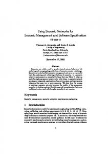
However, despite these tremendous advances, scenario generation remains a challenging problem. The dynamic and time-varying nature of weather, the nonlinear and bounded power conversion processes, and the complex spatial and temporal interactions make model-based approaches difficult to apply and hard to scale, especially when multiple renewable power plants are considered. These models are typically constructed based on statistical assumptions that may not hold or difficult to test in practice, and sampling from high-dimensional distributions (e.g. non-Gaussian) is also nontrivial [3]. In addition, some of these methods depend on certain probabilistic forecasts as inputs, which may limit the diversity of the generated scenarios and under-explore the overall variability of renewable resources. To overcome these difficulties, in this work, we propose a data-driven (or model-free) approach by adopting generative methods. Specifically, we propose to utilize the power of the recently discovered machine learning concept of Generative Adversarial Networks (GANs) [16] to fulfill the task of scenario generation. Generative models has became a research frontier in computer vision and machine learning area, with the promise of utilizing large volumes of unlabeled training data. There are two key benefits of applying such class of methods. The first is that they can directly generate new scenarios based on historical data, without explicitly specifying a model or fitting probability distributions. The second is that they use unsupervised learning, avoiding cumbersome manual labellings that are sometimes impossible for large datasets. In the image processing community, GANs are able to generate realistic images that are of far better quality compared to other methods [16], [17], [18]. In this paper, we show that GANs can also effectively generate renewable scenarios, with suitable modifications that takes into account the fact that renewable resources are driven by physical processes and have different characteristics compared to images. Fig. 1 shows examples of our generated daily scenarios with a comparison (a) 16

4.5

Solar Power (MW)

14

WindPower (MW)

(b) 5

Real Generated

12

3.5

10 8

2

1.5

4

1

2

Fig. 1.

3

2.5

6

0

4

Real Generated

0.5 0

50

100

150

Time (5 mins)

200

250

00

50

100

150

Time (5 mins)

200

250

Group of historical scenarios versus generated scenarios using our method for wind (left) and solar (right) power generation. Blue

curves are true historical data and red curves are generated scenarios. Both scenarios exhibit rapid variation and strong diurnal patterns that are hallmarks of wind and solar power.

to historical scenarios. These generated scenarios correctly capture the rapid variations and strong diurnal cycles in wind and solar. Note we explicitly chose examples where the historical data and the generated scenarios do not match each other perfectly. Our goal is to generate new and distinct scenarios that capture the intrinsic features of the historical data, but not to simply memorize the training data. More examples are shown later in the paper (Fig. 3), and we conduct a host of tests to show that the generated scenarios have the same visual and statistical

August 1, 2017

DRAFT

3

properties as historical data. The intuition behind GANs is to leverage the power of deep neural networks (DNNs) to both express complex nonlinear relationships (the generator) as well as classify complex signals (the discriminator). The key insight of GAN is to set up a the minimax two player game between the generator DNN and the discriminator DNN (thus the use of “adversarial” in the name). During each training epoch, the generator updates its weights to generate “fake” samples trying to “fool” the discriminator network, while the discriminator tries to tell the difference between true historical samples and generated samples. In theory, at reaching the Nash equilibrium, the optimal solution of GANs will provide us a generator that can exactly recover the distribution of the real data so that the discriminator would be unable to tell whether a sample came from the generator or from the historical training data. At this point, generated scenarios are indistinguishable from real historical data, and are thus as realistic as possible. Fig. 2 shows the general architecture of a GANs’ training procedure under our specific setting. 0.05

16

0

0

Historical samples

Output prediction

16 0

50 100 150 200 250

...

50 100 150 200 250

...

0

16 0

50 100 150 200 250

00

20

40

60

80

Discriminator

...

...

Noise input

... ... ... ...

Generated samples 16

... ... ... ...

1

00

50 100 150 200 250

50 100 150 200 250

...

00

real/fake 0

...

16

0 0 50 100 150 200 250

100

Generator Fig. 2.

The architecture for GANs used for wind scenario generation. The input to the generator is noise that comes from an

easily sampled distribution (e.g., Gaussian), and the generator transforms the noise through the DNN with the goal of making its output to have the same characteristics as the real historical data. The discriminator has two sources of inputs, the “real” historical data and the generator data, and tries to distinguish between them. After training is completed, the generator can produce samples with the same distribution as the real data, without efforts to explicitly model this distribution.

The main contributions of this paper are: 1) Data-driven scenario generation: We propose a model-free, data-driven and scalable approach for renewables scenario generation. By employing generative adversarial networks, we can generate scenarios which capture the spatial and temporal correlations of renewable power plants. To our knowledge, this is the first work applying deep generative models to stochastic power generation processes. 2) Conditional scenario generations: We enable generation of scenarios of specific characteristics (e.g., high wind days, seasonal solar outputs) by using a simple label in the training process. This procedure could be easily adjusted to capture different conditions of interest.

August 1, 2017

DRAFT

4

3) Efficient algorithms: We show GANs can be trained with little or no manual adjustments, and it can be swiftly scaled up to generate large and diverse set of renewable profiles. All of the code and data described in this paper are publicly available at https://github.com/chennnnnyize/ Renewables Scenario Gen GAN. The rest of the paper is organized as follows: Section II rigorously formulates the mathematical problems; Section III proposes and describes the GANs model; results are illustrated and evaluated in Section IV; and Section V concludes the paper. II. P ROBLEM F ORMULATION In this section, we give the mathematical formulations for three scenario generation tasks of interest: 1) scenario generation for single renewable resource; 2) scenario generation for multiple correlated renwable resources; and 3) scenario generation conditioned on different events. A. Single Time-Series Scenario Generation Consider a set of historical data for a group of renewable resources at N sites. For site j, let x j be the vector of historical data indexed by time, t = 1, . . . , T , and j ranges from 1 to N. Our objective is to train a generative model based on GANs by utilizing historical power generation data {x j }, j = 1, . . . , N as the training set. Generated scenarios should be capable of describing the same stochastic processes as training samples and exhibiting a variety of different modes representing all possible variations and patterns seen during training. B. Scenario Generation for Multiple Sites In a large system, multiple renewable resources needs to be considered at the same time. Here we are interested in simultaneously generating multiple scenarios for a given group of geographical close sites. We have historical power generation observations {x j }, j = 1, . . . , N for N sites of interests with the same time horizon. The generated scenarios should capture both the temporal and spatial correlations between the resources, as well as the marginal distribution of each individual resource. In some situations a point forecast is given and scenarios should be thought as the forecasting error. Our approach can be easily applied by simply replacing the training samples with the historical forecast errors. Based on different forecasting technologies, there may or may not be correlations among the errors. Our approach would automatically generate statistically correct scenarios without any explicit assumptions. C. Event-Based Scenario Generation In addition to the standard scenario generation process described above, we may want to generate scenarios with distinct properties. For instance, an operator may be interested in scenarios that capture the solar output of a hot summer day. We incorporate these given properties into the training process by labeling each training samples with an assigned label to represent the event. Specifically, we use a label vector y to classify and record certain properties in an observation x j .

August 1, 2017

DRAFT

5

Thus in this part we are interested in scenario generation conditioned on the label y, while samples having same label should follow the similar properties. Our objective here is to train a generative model based on GANs using historical conditional power generation data {x j |y j }, j = 1, . . . , N as a training set. III. G ENERATIVE A DVERSARIAL N ETWORKS In this section, we introduce the GANs [16] and how they are adapted to our applications of interest for renewables scenario generation. We first review the method and formulate the objectives as well as the loss functions, then describe how to incorporate additional information into the model training process. A. GANs with Wasserstein Distance The architecture of GANs we use is shown in Fig. 2. Assume observations xtj for times t ∈ T of renewable power are available for each power plant j, j = 1, ..., N. Let the true distribution of the observation be denoted by pdata (x), which is of course unknown. Suppose we have access to a group of noise vector input z under a known distribution z ∼ pz (z) that is easily sampled from (e.g., jointly Gaussian). Our goal is to transform a sample z drawn from pz such that it follows pdata (x) (without ever learning pdata explicitly). This is accomplished by simultaneously training two deep neural networks: the generator network G(z; θ (G) ) and the discriminator network D(x; θ (D) ). Here, θ (G) and θ (D) are the weights of two neural networks, respectively. For convenience, we sometimes suppress the symbol θ. Generator: During the training process, the generator is trained to take a batch of inputs from the noisy distribution pz (z), and by taking a series of up-sampling operations by neurons of different functions, and output scenarios. Ideally, they should appear as if drawn from pdata . Therefore, after training finishes, the mapping: G(z; θ (G) ) : z → pG (z)

(1)

produces pG (z) that follows the true data distribution pdata (x). Discriminator: The discriminator is trained simultaneously with the generator. It takes input samples either coming from real historical data or coming from generator, and by taking a series of operations of down-sampling using another deep neural network, it outputs a continuous value preal that measures to what extent the input samples belong to pdata (x). The discriminator can be expressed as D(x; θ (D) ) : x → preal

(2)

where x may come from pdata (x) or pG (z). The discriminator is trained to learn to distinguish between pdata (x) from pG (z), and thus to maximize the difference between D(x) (x from real data) and D(G(z)). With the objectives for discriminator and generator defined, we need to formulate loss function LG for generator and LD for discriminator to train them (i.e., update neural networks’ weights based on the losses). In order to set up the game between G and D so that they can be trained simultaneously, we also need to construct a game’s value function V (G, D). A small LG shall reflect G(z) is as realistic as possible from the discriminator’s perspective, e.g., the generated scenarios are looking like historical scenarios for the discriminator. Similarly, a small LD indicates

August 1, 2017

DRAFT

6

discriminator is good at telling the difference between generated scenarios and historical scenarios, which reflect there is a large difference between pG (z) and pdata (x). Following this guideline and the loss defined in [19], we can write LD and LG as followed: LG = −Ez∼pz (z) [D(G(z))]

(3a)

LD = −Ex∼pdata (x) [D(x)] + Ez∼pz (z) [D(G(z))].

(3b)

In the above, the expectations are taken as empirical averages based either on the historical data or on the generated data. Note the functions D and G are parametrized by the weights of the neural networks. We then combine (3a) and (3b) to form a two-player minimax game with the value function V (G, D): min max V (G, D) = Ex∼pdata (x) [D(x)] − Ez∼pz (z) [D(G(z))] G

D

(4)

where V (G, D) is the negative of LD . At early stage of training, G just generates scenario samples G(z) totally different from samples in pdata (x), and discriminator can reject these samples with high confidence. In that case, LD is small, and LG , V (G, D) are both large. The generator gradually learns to generate samples that could let D output high confidence to be true, while at the same time the discriminator is also trained to distinguish these newly fed generated samples from G. As training moves on and goes near to the optimal solution, G is able to generate samples that look as realistic as real data with a small LG value, while D is unable to distinguish G(z) from pdata (x) with large LD . Eventually, we are able to learn an unsupervised representation of the probability distribution of renewables scenarios from the output of G. More formally, the minimax objective (4) of the game can be interpreted as the dual of the so-called Wasserstein distance (Earth-Mover distance) [20]. Given two random variables X and Y with marginal distribution fX and fY , respectively, let Γ denote the set of all possible joint distributions that has marginals of fX and fY . Wasserstein distance between them is defined as Z

W (X,Y ) = inf

fXY ∈Γ

|x − y| fXY (x, y)dxdy.

(5)

This distance, although technical, measures the effort (or “cost”) needed to transport the probability distribution of X to the probability distribution of Y : the inf in (5) finds the joint distribution that gets x and y to have smallest distance while maintaining the marginals [21]. The connection to GANs comes from the fact that we are precisely trying to get two distributions, pdata (D(x)) and pz (D(G(z))) to be close to each other. It turns out that W (D(x), D(G(z))) = sup{Ex∼pdata (x) [D(x)] − Ez∼pz (z) [D(G(z))],

(6)

D

where the expectations can be computed as empirical means. Once the Wasserstein distance we estimate using 4 stops decreasing or reaches pre-set limits, the “cost” of transforming a generated sample to original sample has been minimized, thus we find the optimal generator G∗ . In the GANs community, there is a growing body of literature about the choice of loss functions. Here we chose to use the Wasserstein distance [19] instead of the original Jensen-Shannon divergence proposed in [16] mainly because it allows us to capture all of the modes in the training sample. Training using Jensen-Shannon divergence

August 1, 2017

DRAFT

7

tends to lead the generator to generate a single pattern of power profile that has the highest probability. In this paper, we want to generate scenarios that reflect diverse modes of renewables, which is accomplished by using the Wasserstein distance to directly measure the distance between distributions of real historical data and generated samples. B. Conditional GANs In an unconditioned generative model, we do not control the specific types of the samples being generated by G. Sometimes, we are interested in scenarios “conditioned on” certain class of events, e.g., calm days with intermittent wind, or windy days with farms at full load capacity. Conditional generation is done by incorporating more information to the training procedure of GANs, such that the generated samples conforming to same properties as certain class of training samples. Inspired by supervised learning where we have labels for each training samples, here we propose to combine event labels with training samples, and thus the objective for G is to generate samples under given class [17]. More formally, the problem can be written as: min max V (G, D) = Ex∼pdata (x) [D(x|y)] − Ez∼pz (z) [D(G(z|y))], G

D

(7)

where y encodes different type of classes of conditions. Class labels are assigned based on user-defined classification metrics, such as the mean of daily power generation values, the month of training samples coming from, etc. Note that such class labels are just representation of samples’ events reflected by the power generation data distribution, GANs should be able to learn the conditional distribution and generate samples based on any given meaningful classification metric. We will show the results in Section. IV with given labels based on mean values as well as seasonal information. Since such conditional GANs is only modifying the unconditional GANs model proposed in Section. III-A with a label vector input, both models can be trained using Algorithm 1. In our setup, D(x; θ (D) ) and G(z; θ (G) ) are both differentiable functions which contain different neural layers composed of multilayer perceptron, convolution, normalization, max-pooling and Rectified Linear Units (ReLU). Thus we can use standard training methods (e.g., gradient descent) on these two networks to optimize their performances. Training is implemented in a batch updating style, while a learning rate self-adjustable gradient descent algorithm RMSProp is applied for weights updates in both discriminator and generator neural networks. Clipping is also applied to constrain D(x; θ (D) ) to satisfy certain technical conditions as well as preventing gradients explosion [19]. Detailed model structures and training procedure are described in Section. IV. IV. R ESULTS In this section we illustrate our algorithm on several different setups for wind and solar scenario generation. We first show that the generated scenarios are visually indistinguishable from real historical samples, then we show that they also exhibit the same statistical properties [22], [23]. These results suggest that using GANs would provide an efficient, scalable, and flexible approach for generating high-quality renewable scenarios.

August 1, 2017

DRAFT

8

Algorithm 1 Conditional GANs for Scenario Generation Require: Learning rate α, clipping parameter c, batch size m, Number of iterations for discriminator per generator iteration ndiscri Require: Initial weights θ (D) for discriminator and θ (G) for generator while θ (D) has not converged do for t = 0, ..., ndiscri do # Update parameter for Discriminator Sample batch from historical data: {(x(i) , y(i) )}m i=1 ∼ pdata x Sample batch from Gaussian distribution: {z(i) , y(i) )}m i=1 ∼ pz z Update discriminator nets using gradient descent: (i) (i) gθ (D) ← ∇θ (D) [− m1 ∑m i=1 D(x |y )+ 1 m (i) (i) m ∑i=1 D(G(z |y ))] θ (D) ← θ (D) − α · RMSProp(θ (D) , g

θ (D) )

θ (D) ← clip(w, −c, c) end for # Update parameter for Generator Update generator nets using gradient descent: (i) (i) gθ (G) ← ∇θ (G) m1 ∑m i=1 D(G(z |y ))

θ (G) ← θ (G) − α · RMSProp(θ (G) , gθ (G) ) end while

A. Data Description We build training and validation dataset using power generation data from NREL Wind1 and Solar2 Integration Datasets [24]. The original data has resolution of 5 minutes. We choose 24 wind farms and 32 solar power plants located in the State of Washington to use as the training and validation datasets. All of these power generation sites are of geographical proximity which exhibit correlated (although not completely similar) stochastic behaviors. Our method can easily handle joint generation of scenarios across multiple locations by using historical data from these locations as inputs with no changes to the algorithm. Thus the spatio-temporal relationships are learned automatically. 1 https://www.nrel.gov/grid/wind-integration-data.html 2 https://www.nrel.gov/grid/sind-toolkit.html

August 1, 2017

DRAFT

9

16

Wind 16

(b)

4

6

6

Solar 3

3.5

0 0 16

0 288 0 9

0 0 1

288

0 0 1

−0.1 0

40

0 0

Coefficients

Power(MW)

Auto-corr Generated

Real

Power(MW)

(a) 16

Fig. 3.

0 288 0 16

0 288 0 4

288

00 6

0 288 0 6

0 288 0 3.5

0 288 0 1.5

288

0 288 0 1

0 288 0 1

288

0 0 1

0 288 0 1

0 288 0 1

0 288 0 1

288

40

0 0

0 40 0

0 40 0

0 40 0

40

40

0 0

Time(5mins)

−0.1 40 0

Time(5mins)

Random selected samples from our validation sets (top) versus generated samples from our trained GANs (middle) for

both wind and solar groups. Without using these validation samples in training, our GAN is able to generate samples with similar behaviors and exhibit a diverse range of patterns. The autocorrelation plots (bottom) also verify generated samples’ ability to capture the correct time-correlations.

B. Model Architecture and Details of Training The architecture of our deep convolutional neural network is inspired by the architecture of DCGAN and Wasserstein GAN[18], [19]. The generator G includes 2 de-convolutional layers with stride size of 2 × 2 to firstly up-sample the input noise z, while the discriminator D includes 2 convolutional layers with stride size of 2 × 2 to down-sample a scenario x. The generator starts with fully connected multilayer perceptron for upsampling. The discriminator has a reversed architecture with a single sigmoid output. Details of the generator and discriminator model parameters are listed in the Table I. Note that both G and D are realized as DNN, which can be programmed and trained via standard open source platforms such as Tensorflow [25]. All the program for GANs model is implemented in Python platform with two Nvidia Titan GPUs to accelerate the deep neural networks’ training procedure.3 All models in this paper are trained using RmsProp optimizer with a mini-batch size of 32. All weights for neurons in neural networks were initialized from a centered Normal distribution with standard deviation of 0.02. Batch normalization is adopted before every layer except the input layer to stabilize learning by normalizing the input of every layer to have zero mean and unit variance. With exception of the output layer, Relu activation is used in the generator and Leaky-Relu activation is used in the discriminator. In all experiments, ndiscri was set to 4, so that the model were training alternatively between 4 steps of optimizing D and 1 step of G. We observed model convergence in the loss for discriminator in all the group of experiments. Once the discriminator has converged to similar outputs value for D(G(z)) and D(x), the generator was able to generate realistic power generation samples. 3 Our

code is available at https://github.com/chennnnnyize/Renewables Scenario Gen GAN.

August 1, 2017

DRAFT

10

TABLE I T HE GAN S MODEL STRUCTURE . MLP DENOTES THE MULTILAYER PERCEPTRON FOLLOWED BY NUMBER OF NEURONS ; C ONV /C ONV TRANSPOSE DENOTES THE CONVOLUTIONAL / DECONVOLUTIONAL LAYERS FOLLOWED BY NUMBER OF FILTERS ; S IGMOID IS USED TO CONSTRAIN THE DISCRIMINATOR ’ S OUTPUT IN

Generator G

[0, 1].

Discriminator D

Input

100

24*24

Layer 1

MLP, 2048

Conv, 64

Layer 2

MLP, 1024

Conv, 128

Layer 3

MLP, 128

MLP, 1024

Layer 4

Conv transpose, 128

Sigmoid

Layer 5

Conv transpose, 64

C. Scenario Generation We firstly trained the model to validate that GANs can generate scenario with diurnal patterns. The training evolution for this training dataset is shown in Fig. 4. For the first 10, 000 iterations, the output of discriminator has (a)

D(x)/D(G(z))

Real Gen

Wasserstein Distance

(b)

Fig. 4.

Training evolution for GANs on a wind dataset. (a) The outputs from the discriminator D(x)/D(G(z)) during training

illustrates the evolution of generated samples G(z). At the start, the generated samples (orange) and the real samples (blue) are easily distinguished at the discriminator. As training progresses, they are increasing difficult to distinguish. (b) The empirical Wasserstein distance between the distribution of the real sample and the generated samples, where close to zero means that the two distributions are close to each other.

a large difference between generated and real historical samples, which indicates that the discriminator can easily distinguish between the sources of the samples. However, the final outputs of both D(G(z)) and D(x) converge, which

August 1, 2017

DRAFT

11

indicates that generated samples would exhibit close resemblance to samples from training datasets. Meanwhile, the Wasserstein distance Ex∼pdata (x) [D(x)] − Ez∼pz (z) [D(G(z))] shown in Fig. 4(b) can be used to reflect generated samples’ quality. When it decreases to near-zero, the empirical distribution of a batch of generated scenarios are very close to the empirical distribution of a batch of training scenarios. We then fed the trained generator with 2, 500 noise vector Z drawn from the pre-defined Gaussian distribution z ∼ pz (z). Some generated samples are shown in Fig. 3 with comparison to some samples from the validation set. We see that the generated scenarios closely resemble scenarios from the validation set, which were not used in the training of the GAN. Next, we show that generated scenarios have two important properties: 1) Mode Diversity: The diversity of modes variation are well captured in the generated scenarios. For example, the scenarios exhibit hallmark characteristics of renewable generation profiles: e.g., large peaks, diurnal variations, fast ramps in power, etc. For instance, in the third column in Fig. 3, the validating and generated sample both include sharp changes in its power. Using a traditional model-based approach to capture all of these characteristics would be challenging, and may require significant manual effort. 2) Statistical Resemblance: In addition to visual inspection, we verify that generated scenarios has the same statistical properties as the historical data. For the original and generated samples shown in Fig. 3, we first calculate and compare sample autocorrelation coefficients R(τ) with respect to time-lag τ: E[(St − µ)(St+τ − µ)] (8) σ2 where S represents the stochastic time-series of either generated samples or historical samples with mean µ R(τ) =

and variance σ . Autocorrelation represents the temporal correlation at a renewable resource, and capture the correct temporal behavior is of critical importance to power system operations. The bottom rows of Fig. 3 verify that the real-generated pair have very similar autocorrelation coefficients. In addition to comparing the stochastic behaviors in single time-series, in Fig.5 we show the cumulative distribution function (CDF) of historical and generated samples. We find that the two CDFs nearly lie on top of each other. This indicates the capability of GANs to generate samples with the correct marginal distributions. D. Spatial Correlation Instead of feeding a batch of sample vectors x(i) representing a single site’s diurnal generation profile, here we feed GANs with a real data matrix {x(i) } of size N × T , where N denotes the total number of generation sites, while T denotes the total number of timesteps for each scenario. Here we choose N = 24, T = 24 with a resolution of 1 hour. A group of real scenarios {x(i) } and generated scenarios {G(z(i) )} for the 24 wind farms are ploted in Fig. 6. By visual inspection we find that the generated scenarios retain both the spatial and temporal correlations in the historical data (again, not seen in the training stage). To further validate the quality of generated scenarios, we compute the spatial correlation coefficients and visualize them in Fig. 7. Results show that generated scenarios’ spatial correlation agrees with training sets, even under complex spatial correlation patterns. Thus GANs is able to capture both the spatial and temporal correlations at the same time.

August 1, 2017

DRAFT

12

CDF

(a) 1 0.9 0.8 0.7 0.6 0.5 0.4 0.3 0.2 0.1 0

(b)

Generated Real

0

2

4

6

8

10

Wind Power(MW)

12

1

14

16

Generated Real

0.9 0.8

CDF

0.7 0.6 0.5 0.4 0.3 0.2 0.1 0 0

Fig. 5.

1

2

3

4

5

6

Solar Power (MW)

7

8

9

We evaluate the quality of generated scenarios by calculating the marginal CDFs of generated and historical scenarios

of wind (Figure (a)) and solar (Figure (b)), respectively. The two CDFs are nearly identical for both solar and wind.

E. Conditional Scenario Generation In this setting we are adding class information for the GANs’ training procedure, and the generated samples could be “conditioned” to certain context or statistics informed by such labels. Here we present two representative applications using class information. For a wind data set, we calculate the mean value of power generation for each sample x, and classify these samples into 5 groups based on mean value µ(x) (MW): µ(x) < 0.5, µ(x) < 1.5, µ(x) < 3, µ(x) < 6 and µ(x) ≥ 6. Class information y is encoded as an one-hot (indicator) vector. We then feed the new concatenated vector (x, y) into GANs and train the model using Algorithm 1. We generate a group of 2, 000 wind generation scenarios, with 400 samples in each month. We evaluate these conditional generated samples by verifying the marginal distribution in the range of [0MW, 16MW ] for each class as shown in Fig. 8. The distribution value is divided into 10 equal bins. For each subclass of generated samples, it follows the same marginal distribution as the corresponding training samples. For instance, within the class of µ(x) < 0.5, generated samples’ distribution informs us that it is unlikely to have large values of power generation. While in the class of µ(x) ≥ 6, over 30% of samples’ generation value lies in the interval of [14.4MW, 16MW ], which can be used to simulate targeted high wind days.

August 1, 2017

DRAFT

13

Power Value(MW)

(a) Real 16 14 12 10 8 6 4 2 00 5 (b) Generated 16 14 12 10 8 6 4 2 0 0 5

20

10 15 Time(Hours)

20

Power Value(MW)

10 15 Time(Hours)

Fig. 6.

A group of one-day training (top) and generated (bottom) wind farm power output. The latter behaves similarly to the

former both spatially and temporally.

Real

Generated

1

1

0.9

0.9

5

0.8 0.7

10

0.6 0.5

15

Wind Farms

Wind Farms

5

0.8 0.7

10

0.6 0.5

15

0.4 0.3

20

0.4 0.3

20

0.2

5

10 15 Wind Farms

20

0.1

0.2

5

10 15 Wind Farms

20

0.1

Fig. 7. The spatial correlation coefficients colormap for a group of 24 wind farm one-day training scenarios (left) and generated

scenarios (right). The maps are nearly identical. Samples were shuffled to break the geographical proximity, which make the task of learning spatial correlation more difficult.

For the solar dataset, we add in labels based on month. So y is a 12-dimension one-hot vector indicating which month the sample comes from. By adding this class information, we want to find out GANs is able to characterize the seasonal information reflected by y, e.g., a longer duration of power generation in the summer compared to the winter generation profile. Following the same training procedure as for conditional wind scenario generation, we

August 1, 2017

DRAFT

14

(a) Real 1

0.9

Probability(p.u.)

0.8 0.7 0.6 0.5 0.4 0.3 0.2 0.1 0

1

2

Classes

1

2

Classes

(b) Generated

3

4

5

3

4

5

1

Probability(p.u.)

0.9 0.8 0.7 0.6 0.5 0.4 0.3 0.2 0.1 0

Fig. 8.

The marginal distribution for training scenarios (top) and generated scenarios (bottom) with 5 events (low wind to high

wind) based on wind scenarios’ power generation mean value.

generate a group of 2, 400 solar generation scenarios, with 200 samples in each month.

To verify the generated samples indicate the seasonal patterns, we evaluate both the daily power generation sum values as well as daily power generation duration for each month’s samples. The dry-summer Mediterranean climate existing in most parts of State of Washington is correctly identified by the generated samples, both based on power and duration. Fig. 9 shows the significant difference of daily power generation, while Fig. 10 also agrees with the seasonal variation of sunshine duration. With such scenarios generated based on months, power system operators are able to design seasonal-adaptive renewables dispatch strategies. V. C ONCLUSION AND D ISCUSSIONS Scenario generation can help model the uncertainties and variations in renewables generation, and is an essential tool for decision-making in power grids with high penetration of renewables. In this paper, a novel machine learning model, the Generative Adversarial Networks (GANs) is presented and proposed to be used for scenario generation of renewable resources. Our proposed method is data-driven and model-free. It leverages the power of deep neural

August 1, 2017

DRAFT

15

Real Generated

Daily Power Value(MW)

700 600 500 400 300 200 100 0

Fig. 9.

1

2

3

4

5

6

7

8

Months

9

10

11

12

Seasonal variation of daily power generation values for training and generated solar power generation scenarios. 14

Real Generated

12

Hous(h)

10 8 6 4 2 0

Fig. 10.

1

2

3

4

5

6

7

Months

8

9

10

11

12

Seasonal variation of daily power generation duration for training and generated solar power generation scenarios.

networks and large sets of historical data to perform the task for directly generating scenarios conforming to the same distribution of historical data, without explicitly modeling of the distribution. The case study using proposed model setup shows that GANs works well for scenario generation for both wind and solar. We also show in the simulation that by just retraining the model using historical data from multiple sites samples, GANs are able to generate scenarios for these sites with the corrected spatio-temporal correlations without any additional tuning. We also observe that by adding class information indicating scenario’s properties, GANs is able to generate class-conditional samples conforming to the same sample properties. We validate the quality of generated samples by a series of statistical methods. Since our proposed methodology do not require any particular statistical assumptions, it can be applied to most stochastic processes of interest in power systems. In addition, as the method uses a feed forward neural network structure, it does not require sampling of potentially complex and high dimensional processes and can be scaled easily to systems with a large number of uncertainties. In future work, we propose to incorporate GANs into probabilistic forecasting problems. In addition, we also would like to utilize the scenarios and extend this work to the decision-making strategy design for high penetration of renewables generation.

August 1, 2017

DRAFT

16

R EFERENCES [1] H. Holttinen, P. Meibom, C. Ensslin, L. Hofmann, J. Mccann, J. Pierik et al., “Design and operation of power systems with large amounts of wind power,” in VTT Research Notes 2493.

Citeseer, 2009.

[2] M. R. Patel, Wind and solar power systems: design, analysis, and operation.

CRC press, 2005.

[3] J. M. Morales, R. Minguez, and A. J. Conejo, “A methodology to generate statistically dependent wind speed scenarios,” Applied Energy, vol. 87, no. 3, pp. 843–855, 2010. [4] S. Delikaraoglou and P. Pinson, “High-quality wind power scenario forecasts for decision-making under uncertainty in power systems,” in 13th International Workshop on Large-Scale Integration of Wind Power into Power Systems as well as on Transmission Networks for Offshore Wind Power (WIW 2014), 2014. [5] W. B. Powell and S. Meisel, “Tutorial on stochastic optimization in energy part i: Modeling and policies,” IEEE Transactions on Power Systems, vol. 31, no. 2, pp. 1459–1467, 2016. [6] C. Zhao and Y. Guan, “Unified stochastic and robust unit commitment,” IEEE Transactions on Power Systems, vol. 28, no. 3, pp. 3353–3361, 2013. [7] J. R. Birge and F. Louveaux, Introduction to stochastic programming.

Springer Science & Business Media, 2011.

[8] S. Mitra, “Scenario generation for stochastic programming,” OPTIRISK systems, Tech. Rep., 2006. [9] T. Wang, H.-D. Chiang, and R. Tanabe, “Toward a flexible scenario generation tool for stochastic renewable energy analysis,” in 2016 Power Systems Computation Conference (PSCC), 2016, pp. 1–7. [10] J. E. B. Iversen and P. Pinson, “RESGen: Renewable Energy Scenario Generation Platform,” in Proceedings of IEEE PES General Meeting, 2016. [11] G. Papaefthymiou, P. Schavemaker, L. Van der Sluis, W. Kling, D. Kurowicka, and R. Cooke, “Integration of stochastic generation in power systems,” International Journal of Electrical Power & Energy Systems, vol. 28, no. 9, pp. 655–667, 2006. [12] P. Pinson, H. Madsen, H. A. Nielsen, G. Papaefthymiou, and B. Kl¨ockl, “From probabilistic forecasts to statistical scenarios of short-term wind power production,” Wind energy, vol. 12, no. 1, pp. 51–62, 2009. [13] X.-Y. Ma, Y.-Z. Sun, and H.-L. Fang, “Scenario generation of wind power based on statistical uncertainty and variability,” IEEE Transactions on Sustainable Energy, vol. 4, no. 4, pp. 894–904, 2013. [14] K. Høyland and S. W. Wallace, “Generating scenario trees for multistage decision problems,” Management Science, vol. 47, no. 2, pp. 295–307, 2001. [15] A. Papavasiliou, S. S. Oren, and R. P. O’Neill, “Reserve requirements for wind power integration: A scenario-based stochastic programming framework,” IEEE Transactions on Power Systems, vol. 26, no. 4, pp. 2197–2206, 2011. [16] I. Goodfellow, J. Pouget-Abadie, M. Mirza, B. Xu, D. Warde-Farley, S. Ozair, A. Courville, and Y. Bengio, “Generative adversarial nets,” in Advances in neural information processing systems, 2014, pp. 2672–2680. [17] M. Mirza and S. Osindero, “Conditional generative adversarial nets,” arXiv preprint arXiv:1411.1784, 2014. [18] A. Radford, L. Metz, and S. Chintala, “Unsupervised representation learning with deep convolutional generative adversarial networks,” arXiv preprint arXiv:1511.06434, 2015. [19] M. Arjovsky, S. Chintala, and L. Bottou, “Wasserstein GAN,” arXiv preprint arXiv:1701.07875, 2017. [20] C. Villani, Optimal transport: old and new.

Springer Science & Business Media, 2008, vol. 338.

[21] Y. Rubner, C. Tomasi, and L. J. Guibas, “The earth mover’s distance as a metric for image retrieval,” International journal of computer vision, vol. 40, no. 2, pp. 99–121, 2000. [22] P. Pinson and R. Girard, “Evaluating the quality of scenarios of short-term wind power generation,” Applied Energy, vol. 96, pp. 12–20, 2012. [23] M. Kaut and S. W. Wallace, Evaluation of scenario-generation methods for stochastic programming, J. L. Higle, W. Rmisch, and S. Sen, Eds.

Humboldt-Universitt zu Berlin, Mathematisch-Naturwissenschaftliche Fakultt II, Institut fr Mathematik, 2003.

[24] C. Draxl, A. Clifton, B.-M. Hodge, and J. McCaa, “The wind integration national dataset (wind) toolkit,” Applied Energy, vol. 151, pp. 355–366, 2015. [25] M. Abadi, A. Agarwal, P. Barham, E. Brevdo, Z. Chen, C. Citro, G. S. Corrado, A. Davis, J. Dean, M. Devin et al., “Tensorflow: Large-scale machine learning on heterogeneous distributed systems,” arXiv preprint arXiv:1603.04467, 2016.

August 1, 2017

DRAFT