Object Category Recognition Using Generative

Object Category Recognition Using Generative Template Boosting Shaowu Peng1,3 , Liang Lin2,3 , Jake Porway4, Nong Sang1,3 , and Song-Chun Zhu3,4 1

2

IPRAI, Huazhong University of Science and Technology, Wuhan, 430074, P.R. China. {swpeng, nsang}@hust.edu.cn

School of Information Science and Technology, Beijing Institute of Technology, Beijing, 100081, P.R. China. {linliang}@bit.edu.cn 3

Lotus Hill Institute for Computer Vision and Information Science, Ezhou, 436000, P.R. China. 4

Departments of Statistics, University of California, Los Angeles Los Angeles, California, 90095, USA. {jporway, sczhu}@stat.ucla.edu

Abstract. In this paper, we present a framework for object categorization via sketch graphs, structures that incorporate shape and structure information. In this framework, we integrate the learnable And-Or graph model, a hierarchical structure that combines the reconfigurability of a stochastic context free grammar(SCFG) with the constraints of a Markov random field(MRF), and we sample object configurations as training templates from this generative model. Based on these synthesized templates, four steps of discriminative approaches are adopted for cascaded pruning, while a template matching method is developed for top-down verification. These synthesized templates are sampled from the whole configuration space following the maximum entropy constraints. In contrast to manually choosing data, they have a great ability to represent the variability of each object category. The generalizability and flexibility of our framework is illustrated on 20 categories of sketch-based objects under different scales.

1

Introduction

In the last few years, the problem of recognizing object classes has received growing attention in both the fields of whole image classification[6, 7, 15, 5] and object recognition[1, 14, 16]. The challenge in object categorization is to find class models that are invariant enough to incorporate naturally occurring intra-class variations and yet discriminative enough to distinguish between different classes. In the vision literature, the majority of existing object representations for categorization use local image patches as basic features. These appearance based

2

Shaowu Peng, Liang Lin, Jake Porway, Nong Sang, Song-Chun Zhu

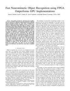
models achieve simple and rich visual/image representations and range from global appearance models (such as PCA) in the 1990s (Nayar et al.)[19], to local representations using invariant feature points (Lowe et al.)[2], patches[12] and fragments[18]. Recently graphical models have been introduced to account for pictorial deformations[11] and shape variances of patches, such as the constellation model[13, 12]. However, these models generally do not account for the large structural or configurational variations exhibited by functional categories, such as vehicles. Other class methods model objects via edge maps, detected boundaries[21, 3],or skeletons[16], which are essential for object representations, but are not designed to deal with large variations, particularly at different scales. Recently, one kind of hierarchical generative model using a stochastic attribute grammar, known as the And-Or graph, was presented by Han[4] and Chen[8]. It is a model that combines the flexibility of a stochastic context free grammar (SCFG) with the constraints of a Markov Random Field (MRF). The And-Or graph models object categories as collections of parts constrained by pairwise relationships. The SCFG component models the probability that hierarchies of object parts will appear and with certain appearances, while the MRF component ensures these parts are arranged meaningfully. More recently, Zhu[17] and Porway[9] defined a probability model on the And-Or graph that allows us to learn its parameters in a unified way for each category. Our categorization framework is built upon a sketch representation of objects along with a learned And-Or graph model for each object category. We sample object configurations from the And-Or graph offline as training templates from which a dictionary of graphlets is learned. Then, four steps of discriminative approaches are adopted to prune candidate categories online, and one graph matching algorithm[10] is developed for top-down verification. The main contribution of this paper is using sampled object templates from the learned And-Or graph model instead of collecting training data manually, and presenting an efficient computing framework for object categorization, integrated with discriminative approaches and top-down verification. Fig. 1 (a) shows the And-Or graph for the bicycle category. The Or-nodes (dashed) are “switching variables”, like nodes in an SCFG, for possible choices of the sub-configurations, and thus account for structural variance.Only one child is assigned to each Or-node during instantiation. The And-nodes (solid) represent pictorial composition of children with certain spatial relations. The relations include butting, hinged, attached, contained, cocentric, colinear, parallel, radial and others constraints. [9] describes how these relations can be effectively pursued in a minimax entropy framework with a small number of training examples. Assigning values to the Or-nodes and estimating the variables on the And-nodes produces various object instances as generated templates. Some examples of the bicycle template are shown in Fig. 1 (b), which can be used as training data in our framework. These templates are synthesized following the maximum entropy principle and are much more uniform than manually collected data would be.

Object Category Recognition Using Generative Template Boosting

3

(b) Synthesized Templates

(a)And-Or graph and-node or-node leaf-node Handle

Seat

Handle 1 Handle 2

Left Handl e

Frame 1

...

...

Stick

Right Handl e

Front Wheel

Frames

...

Frame 2

Frame 3

...

Rear Arm

Frame 4

Rear Wheel

SideVie w

FrontalView

Ellipse Rings

Circle Rings

...

Middle Frame

Front Arm

Fig. 1. A specific object category can be represented by an And-Or graph.(a) shows one example for the bicycle category. An Or-node (dashed) is a “switching variable” for possible choices of the components and only one child is assigned for each object instance. An And-node (solid) represents a composition of children with certain relations. The bold arrows form a sub-graph (also called a parsing graph) that corresponds to a specific object instance (a clock) in the category. The process of object recognition is thus equivalent to assigning values to these Or-nodes to form a “parsing graph”. (b) Several synthesized bicycle instances using the And-Or graph to the left as training data.

In order to show the generalizability and power of categorization using shape and structure information, we use hand-drawn objects, so-called “perfect sketches”, as the testing instances. The remainder of this paper is arranged as follows. We present the principle of synthesizing templates from the And-Or graph model in Section 2. We then follow with a description of the inference schemes, involving discriminative approaches and a top-down matching algorithm[10], along with detailed experiments with comparisons in Section 3. The paper is concluded in Section 4 with a discussion of future work.

2

Generative Template Synthesis

We begin by briefly reviewing the And-Or graph model and then describe the principle of sampling instances from the learned And-Or graph model. The detailed And-Or Graph learning work for each object category was proposed in [9]. 2.1

The Learnable And-Or Graph

The And-Or graph can be formalized as the 6-tuple G =< S, VN , VT , R, P, Σ >

4


where S is the root node, VN are non-terminal nodes for objects and parts, VT are terminal nodes for the atomic description units, R are a set of pairwise relationships, P is the probability model on the graph, and Σ is the set of all valid configurations producible from this graph. In Fig. 1 (a), the root node S is an And node, as bicycle must be expanded into handle, seat, frame, front wheel, rear wheel, while the handle node is an Or node, as only one appearance of handle should exist for each instance of bicycle. Each Or Node Vi OR has a distribution p(ωi ) over which of its ω = {1, 2, ..., N (ωi )} children it will be expanded into. VT = {t1 , t2 , ..., tTn } represents the set of terminal nodes. In our model, the terminal nodes are low-level sketch graphs for object components. They are combined to form more complex nonterminal nodes, as illustrated in Fig. 1 (a). R = {r1 , r2 , ..., rN (R) } in the formulation represents the set of pairwise relationships defined as functions over pairs of nodes vi , vj ∈ VT ∪ VN . rα = ψ α (vi , vj ) each relationship is a function of each node’s attributes, for example the distance between the centers of the two nodes. These relationships are defined at all levels of the tree. P = p(G, Θ) is the probability model over the graph structure. The deriving process of P = p(G, Θ) and the detailed learning process of θ from training set was described in [9]. As the And-Or graph embeds an MRF in a SCFG, it borrows from both of their formulations. We first define the parsing graph as a valid traversal of an And-Or graph, and we then collect a set of parsing graphs labeled from a category of real images as training data to learn the structure and related parameters of the And-Or graph for this category. Each parsing graph will consist of the set of non-terminal nodes visited in the traversal, V = v1 , v2 , ..., vN (v) ∈ VN , a set of resulting terminal nodes T = t1 , t2 , ..., tN (t) ∈ VT , and a set of relationships observed between parts, R ∈ R. Following the SCFG[23], the structural components of the And-Or graph can be expressed as a parsing tree, and its prior model follows the product of all the switch variables ωi at the Or nodes visited. Y p(T ) = pi (ωi ) i∈V

Let p(ωi ) be the probability distribution over the switch variable ωi at node ViOR , θij be the probability that ωi takes value j, and nij the number of times we observe this production, we can rewrite p(T ) as p(T ) =

Y

Y

N (ωi ) n

θijij

i∈V OR j=1

The MRF is defined as a probability on the configurations of the resulting parts of the parsing tree. It can be written in terms of the pairwise energies between parts. We can extend these energies to include constraints on the singleton


5

nodes, e.g. singleton appearance constraints. p(C) =

P P 1 exp− i∈T φ(ti )− ∈V Z

ψ(vi ,vj )

where φ(ti ) denotes the singleton constraint function corresponding to a singleton relationship, and ψ(vi , vj ) denotes the pairwise constraint corresponding to a pairwise relationship. Following the deriving process of [9], we obtain the final expression of P = 1 p(G, Θ). Suppose the number of times we observe this production is nij , RN is the 2 number of singleton constraints, and RN is the number of pairwise constraints, p(G, Θ) =

1 (Θ)p(T )exp{−E(g)} Z

1

E(g) = log(p(T )) +

RN XX i∈T a=1

αai (φa (ti ))

+

X

2

RN X

b βij (ψ b (vi , vj ))

∈V b=1

where Θ = (θ, α, β) are related parameters of the probability model and can be learned from a few parsing graphs, as proved in [9]. Intuitively, for each object category, the basic structural components (object parts or sub-parts) and corresponding relationships are essential and finite, like the basic words and grammar rules, and thus can be learned from a few typical instances, as illustrated in Fig. 2 (a),(b). Furthermore, a huge number of object configurations can be synthesized from the learned And-Or graph that are representative of the in-class variability of each object category, as illustrated in Fig. 2 (c) . 2.2

Template Synthesise

To generate sample templates from the learned And-Or graph, we first sample the tree structure p(T ) of the And-Or graph. This is done by starting at the root of the And-Or graph and decomposing each node into its children nodes recursively. And Nodes are decomposed into all of their children, while an Or node ViOR selects one of its children to decompose into according to the p(ωi ) learned in [9]. This process is similar to generating a sentence from a SCFG[23] model. This continues until all nodes have decomposed into terminal nodes. The output from this step is a parsing graph of the hierarchy of object parts, though no spatial constraints have been imposed yet. For example, we may have selected certain templates for the wheels, frame, seat, and handle bars of a bike, but we have not yet constrained their relative appearances. To arrange the parts spatially, we use Gibbs sampling to sample new part positions and appearances for each pair of parts. At each iteration, we update the value of each of the relationships that exists between each pair of nodes at the same level in the parsing graph. The parameters for each relationship are inherited from the And-Or graph. A relationship R for a given pair of nodes (vi , vj ) is represented as a histogram in our framework [9], and we can thus calculate the change in energy that would occur if this pair were to take on

6


every value in R. For each r that R can assume, we arrange the parts so that their response for this relationship is r. We then compute the total change in energy for the tree by observing the new values of any relationships R′ that were altered between any pairs (vx , vy ) by this change, including (vi , vj ) and R themselves. This energy is easily calculated by plugging the affected relationship responses into our prior model p(G). We record this energy and then arrange according to the next r. For example, given a parsing graph of a car, we would need to update the relative position between the wheels and the body. This would be just one of the relationships between this pair of parts that we would update during this iteration. To do this, we set the size of the wheels to each possible value that the relative position can take on, and then compute the resulting change in energy of the parsing graph. Any relationships between the body and wheels that depend upon the relative position would be affected, as well as any relationships between other parts that depend on the position of the wheels. Once we have a vector of energies for every possible r for a given pair P under R, we exponentiate to get a probability distribution from which we sample the next value v for this P under R. We then move on to the next pair or next relationship. This process continues for 50 iterations in our experiment, at which point we output the final parsing graph, which contains the hierarchy we selected as well as the spatial arrangements of the parts. This process is described in the algorithm below. 1. Sample the tree structure p(T ) to get a parsing graph. 2. Compute the energy of this tree by calculating the energy of each relationship between each pair of terminals. These begin uniformly distributed. 3. For each pair of parts P (a) For each relationship R between P i. Arrange P so that its response to R is r. ii. For every other pair that shares a part with P and every relationship affected by R, compute new responses. iii. Calculate the change in energy ∆E by plugging these new responses into our energy term. iv. Repeat steps i-iii for each value R can take. v. Normalize the ∆E’s to get a probability distribution. Sample a new value y from it for this P under R. 4. Update all pairs of parts under each relationship to their new values y. This sampling procedure thus selects the new relationship values for the pairs of parts proportional to how much they lower the energy at each iteration. As lowering the energy corresponds to increasing the probability of this tree, we are sampling configurations proportional to their probabilities from our learned model. Once we have a parsing graph with all of the leaf nodes appropriately arranged, we must impose an ordering on the terminal nodes to create an appropriately occluded object. This is a logistic issue that is needed to transform


(a) Instances for And-Or graph learning

(b) And-Or graph for each category

7

(c) New Object configurations

Teapot

Spout

Body

Lid

Handle

Vessel

Clock

Frame

Hands

Hour

Min

Sec

Car

Body

Outline

Light

Wheels

Window

Wheel

Fig. 2. Examples of And-Or graphs for three categories (in (b)), and their selected training instances (in (a)) and corresponding samples (in (c)). And The samples (in (c)) contain new object configurations, compared with the training instances (in (a)). Note that, for the sake of space, the And-Or graphs (in (b)) have been abbreviated. For example, the terminal nodes show only one of the many templates that could have been chosen by the Or Node above.

8


our object from overlapping layers of parts into one connected structure. In our experiment we hard-coded these layer values by part type. For example, teapot spouts are always in front of the teapot base. We are currently experimenting with learning an occlusion relationship between pairs so that we can sample this ordering in the future as well. Once the ordering is determined, intersection points between layers are determined and the individual leaf templates are flattened into one final template. By the end of this process we can produce samples that appear similar to the training data, but vary in the arrangements and configurations of their parts. Figure 2 (c) shows examples of these samples at both high and low resolution, along with the corresponding And-Or graph for that category (Figure 2 (b)). Note that, a few new configurations are synthesized, compared with the training instances (Figure 2 (a)). For our experiments, we produced 50 samples for each category.

3

Inference & Experiments

Using the synthesized templates as training data, we illustrate our framework on classifying sketch graphs into 20 categories. In classifying a given sketch graph g, we utilize four stages of discriminative tests to prune the set of candidate categories it can belong to. These discriminative methods are useful as they are quite computationally fast. Finally, a generative top-down matching method is used for verification. All discriminative approaches work in a cascaded way, meaning each step keeps a few candidate categories and candidate templates from each candidate category for the next step. These discriminative approaches were adopted due to their usefulness in capturing object-specific features, local spatial information, and global information respectively. The verification by top-down template matching operates on this final pruned candidate set. This inference framework will be described in the next subsections. We collect 800 images at multiple scales from 20 categories as testing images from the Lotus Hill Institute’s image database[24], as well as the ground truth sketch graphs for each image. We show a few typical instances in Fig. 3 and measure our categorization results with a confusion matrix. 3.1

Discriminative Prune

We first create a dictionary of atomic graph elements, or graphlets. Graphlets are the most basic components of graphs and consist of topologies such as edges, corners, T-junctions, etc. To create a dictionary of graphlet clusters, we first collect all the sketch templates from all categories. Starting with the edge element as the most basic element, we count the frequency of all graphlets across all graphs. A TPS (Thin Plate Spline) distance is used in the counting process to determine the presence of different graphlets. To consider the detectability of each graphlet, we then use each graphlet as a weak classifier in a compositional


9

Fig. 3. Selected testing images with sketch graphs from Lotus Hill Institute’s image database[24].

boosting algorithm[22]. i

Glet

= {(gi , ωi ), i = 1, ..., 13}

According to their weights, we select the top 13 detectable graphlets, and their distributions in each category are plotted in Fig. 4. Other graphlets are either very rare (occurrence frequency is less than 1.0%) or uniform in every category, and thus are ignored.

Graphlet Detectable Order Cross

airplane

bicycle

clock

couch

bucket

chair

Star L-Junction

cup

front view car

Colinear Y-Junction

glasses

hanger

keyboard

knife

T-Junction Parallel Loop

lamp

laptop

monitor

sissors

table

teapot

side view car

Rectangle Acute Angle 3-Junction

watch

U-Junction Arrow X- axis: graphlets 1. Colinear 2. Parallel 3. L-Junction 4. T-Junction 5. Y-Junction 6. Arrow 7. Cross 8. Star 9. Acute Angle 10. U-Junction 11. Rectangle 12. Loop 13. Degree3-Junction

Fig. 4. The graphlets distributions in each category. The graphlets are listed in order according to detectability.

10


To prune candidate categories for a testing instance, we integrate four steps of discriminative approaches. We use confusion matrix to estimate the true positive rate of categorization. In each step, we keep candidates and plot the confusion matrix of top N candidate categories, which describes whether the true category is in the top N candidate categories. The number N of candidates we keep is empirically determined in the training stage and it helps to guarantee high true positive rate and narrow the computing range of the next step. Estimating this number is straightforward and its description is thus ignored in this paper. Step 1 Category histogram The histogram of graphlets for each category is learned by counting graphlet frequency over the training templates. Each testing graph can then be converted into a sparse histogram and the likelihood of its histogram against each category histogram can be calculated for classification. The results of step 1 are shown in Fig. 5 and the top 10 candidates are selected for step 2.

Fig. 5. Step 1 discriminative prune. Three confusion matrix show results with the top 1, top5 and top10 candidate categories. We keep the top 10 candidates for step 2.

Step 2 Nearest Neighbor Each instance in the training data and our testing graph are converted into sparse vectors. Each vector represents the frequency of each graphlet along with its weight. Suppose we have M training templates in each category, then each vector is Vj = {ωi ∗ Ni , i = 1, ..., 13}, j = 1, ..., M Where ωi and Ni are graphlet gi ’s weight and occurrence frequency in template j. To get a distance between two sparse vector, we use a modified Hamming Distance, the L1-Norm of two vectors’ subtraction. Firstly we calculate the distance between our testing instance and each training instance from the 10 candidate categories kept from step 1. Then we find the 8 shortest distances within each category and calculate the average distance between them. The candidate categories can then be ordered by the length of these average distances. We keep the 8 closest candidate categories and 10 closest candidate templates within these categories for step 3, the results of which are shown in Fig. 6. Step 3 Nearest Neighborhood via Composite Graphlet We next introduce spatial information into our features. To capture informative attributes


11

Fig. 6. Step 2 discriminative prune. Three confusion matrix show results with the top 1, top4 and top8 candidate categories. We keep the top 8 candidates for step 3.

of a graph, adjacent graphlets are composed into cliques of graphlets. The training and testing templates can be decomposed into these graphlet cliques and then vectorized for further pruning. The composite graphlets selection work is similar to single graph selection, and the top 20 detectable composite graphlets are shown in Fig. 7. The distance metric is computed in a similar fashion to step 2. We then keep the top 6 candidate categories and top 8 candidate templates from our remaining set, as shown in Fig. 8. Graphlet Detectable Order

airplane

bicycle

bucket

clock

couch

cup

glasses

hanger

keyboard

lamp

laptop

monitor

scissors

table

teapot

chair

Arrow-L ArrowArrow Y-Arrow Y-L

front view car

Cross-Cross Arrow-Cross Y-Cross T-Cross

knife

Y-Y Double-L 2 Y-Colinear Arrow-Colinear

side view car

T-Y Double-L 1 Double-L 3 T-Arrow

watch

T-T T-L T-Colinear PI-Junction X-axis graphlets: 1. PI-Junction 2. Double-L 1 3. Double-L 2 4. Double-L 3 5. T-L 6. T-T 7. T-Y 8. T-Arrow 9. T-Colinear 10. T-Cross 11. Y-L 12. Y-Y 13. Y-Arrow 14. Y-Colinear 15. Y-Cross 16. Arrow-L 17. Arrow-Arrow 18. Arrow-Colinear 19. Arrow-Cross 20. Cross-Cross

Fig. 7. Top 20 detectable composite graphlets and their distributions

Step 4 Nearest Neighborhood via Shape Context Shape context[20] can be considered as one kind of global shape descriptor. It can be used to further prune the candidates proposed by previous steps. We keep the top 5 candidate categories and top 5 candidate templates from each category in this step, as shown in Fig. 9.

12


Fig. 8. Step 3 discriminative prune. Three confusion matrices show results with the top 1, 3, 6 candidate categories. We keep the top 8 candidate templates for step 4.

Fig. 9. Step 2 discriminative prune. Three confusion matrix show results with the top 1, top3 and top5 candidate categories. We keep the top 5 candidates for top-down verification.

3.2

Top-Down verification

Given the results of our cascade of discriminative tests, the template matching process is then activated for top-down verification. The matching algorithm we adopted is a stochastic layered matching algorithm with topology editing that tolerates geometric deformations and some structural differences [10]. As shown in Fig. 10, the final candidate categories and templates for testing objects are listed, and top-down matching is illustrated. The input testing image and its perfect sketch graph are shown in Fig. 10 (a), in which there are two testing instances, a cup and a teapot. After the discriminative pruning, there are two candidate categories left (cup and pot) with candidate templates for the testing cup, as well for the testing teapot, as listed in Fig. 10 (b). After the top-down matching process, the templates with the best matching energy are verified for the categorization task, as illustrated in Fig. 10 (c). The final confusion matrix on 800 objects is shown in Fig. 11. 3.3

Comparison

For comparison purposes, we discard the generative And-Or graph model and instead collect quadruple the amount of training data as sampled templates from the Lotus Hill Institute’s image database[24]. Based on these hand-collected images along with their sketch graphs (200 images for each category), we infer the same testing instances for categorization as we described above. We just


candidate templates

(a)

(b)

13

Top-down verification

(c)

Fig. 10. The top-down verification of candidate templates. The input testing image and its perfect sketch graph are shown in (a), where there are two testing instances, a cup and a teapot. After the discriminative prune there are two candidate categories remaining (cup and teapot) with candidate templates for the testing cup, as well for the testing teapot, as listed in (b). After the top-down matching process, the templates with the best matching energy are verified, as illustrated in (c).

1. airplane 2. bicycle 3. bucket 4. chair 5. clock 6. couch 7. cup 8. front-view car 9. glasses 10. hanger 11. keyboard 12. knife 13. lamp 14. laptop 15. monitor 16. side-view car 17. scissors 18. table 19. teapot 20. watch

Fig. 11. The final confusion matrix on 800 objects.

14


plotted the final confusion matrix for illustration, as shown in Fig. 12. With the same inference steps and testing instances, the overall classification accuracy is 21.5% lower than inference using the generative And-Or graph model. The essential reason for comparison results is that most categories include a nearly infinite number of configurations, which are impossible to cover completely by hand-collected data. Comparison: 1. airplane 2. bicycle 3. bucket 4. chair 5. clock 6. couch 7. cup 8. front-view car 9. glasses 10. hanger 11. keyboard 12. knife 13. lamp 14. laptop 15. monitor 16. side-view car 17. scissors 18. table 19. teapot 20. watch

Fig. 12. Confusion matrix showing the overall classification accuracy of the test categories using training data from hand-collected images. Compared with Fig. 11, it shows numerically that the manually collected training data are of less powerful in representing varied object configurations.

4

Summary

In this paper, a framework composed of a generative And-Or graph model, a set of discriminative tests and a top-down matching method, is proposed for a sketch-based object categorization task. Instead of collecting training data manually, we synthesize object configurations as object templates from the And-Or graph model. In the computational process, four steps of discriminative pruning are adopted to narrow down possible matches, and a template matching algorithm is used on the final candidates for verification. We show detailed experiments of classifying testing sketch graphs into 20 categories step by step. In order to show the generalizability and power of this method, we use the humanannotated sketch graphs as testing instances. With the experimental results and comparisons, the synthesized templates show their ability to represent object with large variability in appearance, and the compositional inference shows their efficiency and accuracy with the experiments results. To get a better performance on words clustering and generative model, we currently focus on objects in form of manually drawn sketch graph. In future, further work about imperfect sketch recognition will be done on pixel images, new model of sketch extraction and object detection will be consider.


5

15

Acknowledgment

This work is done when the authors are at the Lotus Hill Research Institute. The project is supported by Hi-Tech Research and Development Program of China (National 863 Program, Grant No. 2006AA01Z339 and No. 2006AA01Z121) and National Natural Science Foundation of China (Grant No. 60673198 and No. 60672162).

References 1. A. Berg, T. Berg, and J. Malik: Shape Matching and Object Recognition using Low Distortion Correspondence, CVPR, 2005. 2. D. G. Lowe: Distinctive image features from scaleinvariant keypoints, IJCV, 60(2), pp. 91-110, 2004. 3. F. Estrada and A. Jepson: Perceptual Grouping for Contour Extraction, ICPR, 2004. 4. F. Han and S.C. Zhu: Bottom-up/top-down image parsing by attribute graph grammar, ICCV, 2005. 2 5. F. Jurie and B. Triggs: Creating Efficient Codebooks for Visual Recognition, ICCV, 2005. 6. G. Csurka, C. Dance, L. Fan, J. Willamowski, and C. Bray: Visual Categorization with Bags of Keypoints, SLCV workshop in conjunction with ECCV, 2004. 7. G. Dorko and C. Schmid: Selection of Scale-Invariant Parts for Object Class Recognition, ICCV, 2003. 8. H. Chen, Z. Xu, Z. Liu, and S.C. Zhu: Composite Templates for Cloth Modeling and Sketching, CVPR, (1) pp 943-950, 2006. 9. J. Porway, Z. Yao, and S.C. Zhu: Learning an and-or graph for modeling and recognizing object categories, submitted to CVPR 2007, NO. 1892. 10. L. Lin, S.C. Zhu, and Y. Wang: Layered Graph Match with Graph Editing, submitted to CVPR 2007, NO. 2755. 11. M. Fischler and R. Elschlager: The representation and matching of pictorial structures, IEEE Transactions on Computers, 22(1):67C92, 1973. 12. M. Weber, M. Welling, and P. Perona: Towards automatic discovery of object categories, CVPR, 2000. 13. P. Felzenszwalb and D. Hut tenlocher: Pictorial Structures for Object Recognition, IJCV 61(1), pp. 55-79, 2005. 14. P. Viola and M. Jones: Rapid Object Detection using a Boosted Cascade of Simple Features, CVPR, 2001. 15. R. Fergus, P. Perona, and A. Zisserman: Object class recognition by unsupervised scaleinvariant learning, CVPR, 2003. 16. S. C. Zhu and A. L. Yuille: Forms: A flexible object recognition and modeling system. IJCV, 20(3):187C212, 1996. 17. S.C. Zhu and D. Mumford: Quest for a Stochastic Grammar of Images, Foundations and Trends in Computer Graphics and Vision, 2007(To appear). 18. S. Ullman, E. Sali, and M. Vidal-Naquet: A Fragment-Based Approach to Object Representation and Classification, Proc. 4th Intl Workshop on Visual Form, Capri, Italy, 2001. 19. S. K. Nayar, H. Murase, and S. A. Nene: Parametric Appearance Representation, in S. K. Nayar and T. Poggio, (eds) Early Visual Learning, 1996.

16


20. S. Belongie, J. Malik, and J. Puzicha: Shape matching and object recognition using shape contexts. PAMI, 24(4):509C 522, 2002. 21. V. Ferrari, T. Tuytelaars, and L. Van Gool: Object Detection by Contour Segment Networks, ECCV, 2006; 22. Z.W. Tu: Probabilistic Boosting Tree: Learning Discriminative Models for Classification, Recognition, and Clustering, ICCV, 2005. 23. Z. Chi, S. Geman: Estimation of probabilistic context-free grammars, Computational Linguistics, v.24 n.2, 1998. 24. Z. Yao, X. Yang, and S.C. Zhu: An Integrated Image Annotation Tool and Large Scale Ground Truth Database, submitted to CVPR 2007, NO. 1407.