proach for the development of avionic and automotive em- bedded systems. ... tax, all modeling constructs for software and hardware com- ponents needed ...
Model-level Simulation for COLA Markus Herrmannsdoerfer, Wolfgang Haberl, Uwe Baumgarten Institut f¨ur Informatik Technische Universit¨at M¨unchen Boltzmannstr. 3, 85748 Garching b. M¨unchen, Germany {herrmama, haberl, baumgaru}@in.tum.de
Abstract Model-driven development has become the standard approach for the development of avionic and automotive embedded systems. When a semantically founded modeling language is employed, the implemented systems can be checked and further processed in an automated manner. To this end, the Component Language (COLA) was invented. It allows for the definition of all information needed during system development. For a better understanding, and also debugging, of the systems modeled therewith, simulation at the level of the model is a welcome complement. In this paper we present a model-level simulator for COLA. It follows the language’s semantics closely, thus guaranteeing the same behavior as specified in the model and implemented by other tools based on COLA. Furthermore, its modular nature allows for the use of different sources for input data. We will demonstrate the architecture and abilities of our simulator, using parts of a recent case study throughout the paper.
1
Introduction
With the ever growing number of embedded systems — about 90% of all processors are nowadays used in this domain [11] — these systems are expanding into more and more areas of everyday life. This includes consumer electronics as well as safety-critical systems of the avionics and automotive domain. In contrast to the former one, a failure in an avionic or automotive system can cause huge financial damage and, even more fatal, endanger human lives. Besides the demands regarding errors in the development of those hard real-time embedded systems, their usually distributed nature makes things even more complex and an additional source of possible faults. Model-driven development has evolved as a state-ofthe-art approach to tackle these problems. Besides reduced complexity apparent to the developer by the abstrac-
tion used at model-level, a modeling language containing a mathematically defined semantics allows for automated model-checking and verification, which raises the results’ quality even further. Unfortunately, many of the existing approaches lack such a semantic foundation. Additionally, they are also mainly aimed at the definition of partial functionality of a system, leaving aside the integration of different features and the distributed nature of the underlying execution platform. The development of COLA, the Component Language, as we described in [7], was initiated to solve these shortcomings. Offering an easily understandable graphical syntax, all modeling constructs for software and hardware components needed during system development, and a formally defined semantics, the automatic generation of high quality systems from models specified in COLA is made possible. We presented some of the concepts and tools necessary for automatic system generation in [5] and [6]. Still we found it desirable to have a possibility to validate the behavior of a COLA model, especially when changes are made to it, without having to generate code for each test. To this end, we developed the model-level simulator described here. It strictly follows the COLA semantics, thus guaranteeing to behave exactly as the target system. The resulting model-level simulation allows for shorter turnaround times in case of necessary model changes. A key concept of the simulator is its modular architecture. This architecture enables an easy integration of different input data sources for the simulation. So, the simulator described here is able to evaluate models based on user input, generated test data, and even data captured via a logging mechanism in an actual running system. We will showcase the application of the simulator using several examples taken from a case study we recently implemented in COLA. The implemented functionality is that of a parking assistant system, enabling a car to park automatically. The case study was carried out using a model car equipped with three computing nodes and several sensors for measur-
ing distances. We will give more detail on the case study throughout the paper.
right_back right [32] distance_front_right distance_right
Outline. Section 2 provides an overview of the modeling language COLA the simulator was realized for. Our approach to systematically implement a simulator for COLA is detailed in Section 3. In Section 4, we compare our approach with related work. Finally, we recapitulate the benefits of the presented simulator in Section 5.
2
out
-150
vehicle_steering
back [-6]
out
out
vehicle_speed
vehicle_distance_control
axle_rotation
right_back [22]
wanted_axle_rotations reset
current_step out
axle_rotation ready
ready
reset
goto_next
goto_next
Figure 1. Example Network.
Overview of COLA
COLA is a modeling language for the design of distributed, safety-critical real-time systems. COLA is based on the synchronous data-flow paradigm and has a welldefined semantics (cf. [7]). An excerpt of the COLA metamodel is depicted on the left side of Figure 5. The key concept of COLA is that of Units. These can be composed hierarchically, or occur in terms of Blocks that define the basic (arithmetic and boolean) functions of an application. Each unit has a set of typed input and output Ports describing its interface. Units can be used to build more complex components by composing a Network of units and by defining an interface to such a network. The sub-units are connected by so-called Channels which connect an output port with one or more suitably typed input ports (cf. [8]). As communication takes no time according to the synchronous paradigm, feedback circles of channels connecting an output port of a network to an input port of the same network have to contain a Delay block which defers propagation by one time interval. Otherwise such a feedback would define a recursive call, which is prohibited in COLA because of the unknown amount of execution time consumed by such a unit. COLA enables the reuse of units within networks by requiring to compose Instances of units. Figure 1 depicts the graphical representation of an example network which implements a part of the parking curve of the case study. In the graphical syntax of COLA, ports are represented by triangles, units and their instances by rounded rectangles, and channels by lines. The unit vehicle distance control is an example for reuse, as it is employed several times within the model. In addition to the hierarchy of networks, COLA provides a decomposition into Automata, i. e., finite state machines, similar to Statecharts [3]. If a unit is decomposed into an automaton, each State of the automaton is associated with a corresponding sub-unit, which determines the behavior in that particular state. This definition of an automaton is therefore well-suited to partition complex networks of units into disjoint operating modes (cf. [2]), the activation of which depends on the input signals of the automaton. In Figure 2 the graphical representation of an example
automaton which defines the different steps of the parking algorithm is given. In the graphical syntax of COLA, states are represented by circles, and transitions by arrows. The network implementing the state right back has been shown in Figure 1. parking
right_back
distance_front_right
vehicle_steering distance_right vehicle_speed axle_rotation
reset
back current_step
reset ready goto_next
left_back
Figure 2. Example Automaton. The collection of all units represents a COLA System, which models the application, possibly including its environment. Such a system does not have any unconnected input or output ports, as there would be no way to provide input to system. For effective communication with the environment not describable within the functional COLA model, Sources and Sinks model connectors to the underlying hardware. Sources are the model representation of sensors, and sinks correspond to actuators of the used hardware platform. The example we use throughout this paper is that of a parking assistant which automatically parks a car. The system observes distance and rotation values from sensors and governs actuators for speed and steering control. To showcase our approach, the parking assistant was tested in a model car which is depicted in Figure 3. The model car is able to run in parallel to a wall, and use a detected gap of sufficient length as parking space. The simulator was a great help during the debugging of the modeled system, showing the impact of model changes right away – without the need to generate code and deploy it onto the demonstrator for each minor change in the model.
Design Model
Runtime Model
Port inPorts *
1 valuation * outPorts
* valuations 1 node
Unit
1 unit
Valuation value
1 unit
Node state * children
Block
Network
Automaton
* instances
Instance
Figure 3. Case Study. Design Model decorates
Runtime Model
Environment Model
operates on
operates on
Execution Model
Figure 4. Architecture of the Simulator.
3
SubUnit
1 edge
Figure 5. Metamodel of Design and Runtime Model.
derive
Simulator
* states
State
Simulator Architecture
The simulator allows to execute a COLA system at the abstraction level of the model. This so-called design model which is designed by the software engineer using COLA, serves as input to the simulator. The architecture of the simulator is depicted in Figure 4. For flexibility, we modularized the architecture into three components: the runtime model, the environment model, and the execution model. The runtime model describes the runtime configuration of a system. That means, it decorates the design model with information required at runtime, for example states of automata or delays. The initial runtime model can be automatically derived from the design model. This transformation is described, together with the structure of the runtime model, in Section 3.1. The environment model specifies the behavior of the environment surrounding the system. Therefore, it controls the inputs and observes the outputs at the system’s boundary by simulating sources and sinks. It depends on the kind of environment model whether there is a feedback from outputs to inputs. The interface of the environment model and its possible implementations are described in Section 3.2. The execution model performs a stepwise execution of the system. This is done by modifying the runtime model
depending on the inputs and generating the outputs at the system’s boundary. The execution model is determined by the semantics of the modeling language. Section 3.3 illustrates how the execution model operates on both runtime and environment model.
3.1
Runtime Model
The runtime model describes the runtime configuration of a system and is derived from the design model. The additions to the metamodel employed by the runtime model are depicted on the right hand side of Figure 5. The runtime model has to extend the design model with a state at runtime. The current state has to be maintained for all stateful units, i. e. automata and delays. Furthermore, we also memorize the Valuations of input and output ports for each unit. As a consequence, the execution model is able to store intermediate results during execution. These intermediate results are displayed in the simulator’s graphical user interface (GUI) for visualization. Figure 7 gives an impression of the realized GUI: states currently active within automata are highlighted, and ports are accompanied by their current valuation. As we already explained in Section 2, COLA provides a mechanism to reuse units in the design model. The structure of a design model is thus basically a directed acyclic graph, with units being the nodes and the hierarchical composition relation being the edges. For the reasons explained below, the runtime model has to follow a slightly different structure. Figure 6 compares the runtime model to its corresponding design model for our running example. While squared rectangles denote networks and solid arrows denote their instances, automata are represented by rounded rectangles and their states by dashed arrows.
right_back
Design Model
Runtime Model
parking
parking
back
left_back
reset
distance
right_back
back
left_back
distance
distance
distance
reset
... sum
abs
sum
abs
abs
sum
abs
abs
Figure 6. Example of Design Model and Runtime Model. The left half of Figure 6 depicts the design model structure for the automaton responsible for parking the car. Networks distance and abs are reused three and two times, respectively. This is indicated by the multiple incoming arrows. However, different instances of the very same unit may be in different states at runtime. As a consequence, these states have to be maintained separately by the runtime model. In order to do so, we have to unfold the structure of the design model such that the runtime model is basically a tree. The right hand side of Figure 6 shows the structure of the corresponding runtime model for the parking automaton. The runtime model now contains three nodes of the network distance, and even six nodes of the network abs, as it is reused within a reused unit. We sometimes wish to modify the design model in order to fix errors identified during simulation. To validate whether the modification actually fixes the error, it is desirable to continue simulation afterwards rather than restarting it. However, the runtime model needs to co-evolve with the design model to be able to continue simulation. This problem can be solved by incremental transformation: the runtime model needs to listen to, and adapt itself to the changes of the design model. When an instance is added to a network in COLA for example, a sub-tree corresponding to the instance has to be added to the network’s node in the runtime model. We have found this feature very useful and time-saving when debugging our case study.
3.2
Environment Model
The environment model controls the inputs and observes the outputs at the system’s boundary. As a consequence, the environment model only needs to know about the system boundary, namely the sources and sinks of the system. We implemented different kinds of environment models while performing our case study. In the following, we present these environment models and their purpose.
A very simple environment model is required during interactive simulation triggered by a user. The user controls the inputs by entering values and observes the outputs through the simulator GUI. He can thereby validate whether the system performs as intended. A more sophisticated environment model provides feedback from the outputs to the inputs. We have implemented an environment model that maintains the current position of a car and the direction in which it is heading. Position and direction is updated based on the outputs for steering and engine control of the system. The inputs to the system are calculated based on both position and direction and a virtual wall that is given by its coordinates. This environment model allows us to simulate the parking procedure directly at model-level. The middle tab in Figure 7 depicts the visualization of the parking procedure within the simulator GUI. Another environment model was implemented for the model-based generation of test cases. The inputs to the system are randomly generated, and are — together with the outputs — stored in a trace. However, naive random generation of input values would lead to jumps which may not be realistic. Therefore, so-called user profiles provide a means to better control the generation of input values. A user profile for an integer-typed input for instance provides a minimum and maximum value, a probability that the value changes and a range within which the value may change. Finally, traces captured at runtime in a real system modeled with COLA can be executed in the simulator by means of another environment model. A trace is a binary file containing the input and output values, as well as the states of all unit instances, for every execution step on the actual execution platform. The trace environment model provides the values from the trace as input, and verifies whether the outputs from the simulation correspond to the values from the trace. In addition, these traces can be used to verify whether the actual running system corresponds to the model.
Figure 7. Graphical User Interface of the Simulator.
3.3
Execution Model
The execution model performs a stepwise execution of the system. It operates on both the environment model and the runtime model: The execution model obtains the inputs from the environment model, performs an evaluation of the runtime model, and feeds the outputs back to the environment model. The execution model thus reflects the operational semantics of the modeling language. As COLA is a synchronous data-flow language, all units have to be evaluated within one step — except for those that are defined within currently inactive automaton states. During evaluation, the tree that is spanned by the runtime model is visited in a top-down manner. The evaluation of each node in the runtime model depends on the kind of unit to which the node is attached. For a network, the nodes corresponding to the contained units have to be evaluated in a certain order: a topological sorting based on the data dependencies arising from the channels connecting them. As we already mentioned in Section 2, delay blocks have to be excluded from these
dependencies, as they delay propagation by one time interval. For each child node, the values are propagated to its input ports before it is evaluated. After evaluation, the values are available at its output ports for the nodes depending on them, i. e. nodes connected to the ports via channels. The basic blocks of COLA have an implicit meaning, representing arithmetic, boolean, etc., operators, which also has to be implemented by the execution model. Finally, after all instances are evaluated, the values are propagated to output ports of the network. For an automaton, the active state may have to be changed. Therefore, the nodes corresponding to transitions emanating from the current state are evaluated. In case one of them evaluates to true, the current state is changed to the transition’s target state. Only then, the input values are propagated to the state and its node is evaluated. The output values of this state are then propagated as the automaton’s output values. According to its definition, COLA does not allow a model to be defined partially and thus a system has to be deterministic. For requirements modeling, we have de-
fined an extension of COLA that admits partiality. For this extension, we have implemented a separate execution model that allows us to explicitly simulate the resulting nondeterminism. In this execution model, the active automaton state and the port valuations have to be extended from single values to sets of possible values.
on. Finally, data captured in a running system instance can be used as input for debugging purposes. We believe this adaptability to be a key factor for auxiliary simulation, leading to less errors contained in the resulting systems.
4
´ ´ ad Bakay, M. Mar´oti, P. V¨olgyesi, [1] Akos L´edeczi, Arp´ G. Nordstrom, J. Sprinkle, and G. Karsai. Composing domain-specific design environments. Computer, 34(11):44–51, 2001. [2] A. Bauer, M. Broy, J. Romberg, B. Sch¨atz, P. Braun, U. Freund, N. Mata, R. Sandner, and D. Ziegenbein. AutoMoDe — Notations, Methods, and Tools for Model-Based Development of Automotive Software. In Proceedings of the SAE 2005 World Congress, Detroit, MI, April 2005. Society of Automotive Engineers. [3] G. Booch, J. Rumbaugh, and I. Jacobson. The Unified Modeling Language User Guide. Addison-Wesley, 1998. [4] C. Brooks, E. A. Lee, X. Liu, S. Neuendorffer, Y. Zhao, and H. Zheng. Heterogeneous concurrent modeling and design in java (volume 1: Introduction to ptolemy ii). Technical Report UCB/EECS-2008-28, EECS Department, University of California, Berkeley, Apr 2008. [5] W. Haberl, U. Baumgarten, and J. Birke. A Middleware for Model-Based Embedded Systems. In Proceedings of the 2008 International Conference on Embedded Systems and Applications, ESA 2008, Las Vegas, Nevada, USA, July 2008. [6] W. Haberl, M. Tautschnig, and U. Baumgarten. From COLA Models to Distributed Embedded Systems Code. IAENG International Journal of Computer Science, 35(3):427–437, Sept. 2008. [7] S. Kugele, M. Tautschnig, A. Bauer, C. Schallhart, S. Merenda, W. Haberl, C. K¨uhnel, F. M¨uller, Z. Wang, D. Wild, S. Rittmann, and M. Wechs. COLA – The component language. Technical Report TUM-I0714, Institut f¨ur Informatik, Technische Universit¨at M¨unchen, Sept. 2007. [8] C. K¨uhnel, A. Bauer, and M. Tautschnig. Compatibility and reuse in component-based systems via type and unit inference. In Proceedings of the 33rd EUROMICRO Conference on Software Engineering and Advanced Applications (SEAA). IEEE Computer Society Press, 2007. [9] OMG. Meta object facility (mof) 2.0 query/view/transformation specification. Technical report, OMG, 2008. [10] D. A. Sadilek and G. Wachsmuth. Prototyping visual interpreters and debuggers for domain-specific modelling languages. In Model Driven Architecture - Foundations and Applications, volume 5095/2008 of Lecture Notes in Computer Science, pages 63–78. Springer Berlin / Heidelberg, 2008. [11] S. Schulz, J. W. Rozenblit, and K. Buchenrieder. Multilevel testing for design verification of embedded systems. IEEE Design & Test of Computers, 19(2):60–69, 2002.
Related Work
Ptolemy [4] is a tool set for the simulation of heterogeneous systems, i. e. composed of components which may obey different execution models. Similar to our approach, the implementation of a new execution model can be easily added. However, their architecture does not provide a clear separation between design and runtime model. GME [1] is a generic framework for the definition of new modeling languages including a simulator. Akin to our approach, a separate runtime model is created on which the execution model operates. Though the framework does not provide a means to integrate an explicit environment model. EProvide [10] is a framework to prototype visual interpreters and debuggers for modeling languages. Like in our approach, they distinguish between design and runtime model. They make use of the language QVT [9] for model transformation to specify the execution model. In contrast to our work, their framework does not take an explicit environment model into account. All presented approaches rely on a certain framework that provides crucial services to realize a simulator. Using such a framework leads to dependencies on other frameworks, e. g., a certain metamodeling framework, which may not be desired for other reasons. Furthermore, a framework may impose limitations, e. g., concerning the execution model that can be expressed with it. Therefore, we did not want to present yet another framework, but rather a systematic approach towards the realization of a simulator.
5
Conclusions
In this paper we presented our model-level simulator for the Component Language. The simulator is a welcome addition to facilitate the development of systems using COLA as a modeling language. Besides the compliance of the simulator to the defined COLA semantics, thus showing the same behavior as executable code generated from the model, the simulator mainly appeals with its modular architecture. The use of different data sources enables its application during different stages of systems development. While during early development phases only manually chosen input data might be available, the growing knowledge about the system and the employed hardware allows to specify user-profiles for test case generation later
References