Multiscale Methods for Model Order Reduction of Non Linear ...

Multiscale Methods for Model Order Reduction of Non Linear Multiphase Flow Problems

arXiv:1803.03721v1 [math.NA] 9 Mar 2018

Gurpreet Singh

Wingtat Leung

Mary F. Wheeler

March 13, 2018

Abstract Numerical simulations for flow and transport in subsurface porous media often prove computationally prohibitive due to property data availability at multiple spatial scales that can vary by orders of magnitude. A number of model order reduction approaches are available in the existing literature that alleviate this issue by approximating the solution at a coarse scale. We attempt to present a comparison between two such model order reduction techniques, namely: (1) adaptive numerical homogenization and (2) generalized multiscale basis functions. We rely upon a non-linear, multi-phase, black-oil model formulation, commonly encountered in the oil and gas industry, as the basis for comparing the aforementioned two approaches. An expanded mixed finite element formulation is used to separate the spatial scales between non-linear, flow and transport problems. To the author’s knowledge this is the first time these approaches have been described for a practical non-linear, multiphase flow problem of interest. A numerical benchmark is setup using fine scale property information from the 10th SPE comparative project dataset for the purpose of comparing accuracies of these two schemes. An adaptive criterion is employed in by both the schemes for local enrichment that allows us to preserve solution accuracy compared to the fine scale benchmark problem. The numerical results indicate that both schemes are able to adequately capture the fine scale features of the model problem at hand.

1

Introduction

Since the advent of numerical reservoir simulations, oil-field operations have received a substantial boost in confidently predicting recovery estimates and determining operational choices during the deployment of a specific recovery technology. During the screening stage, numerical reservoir models are built and simulations are run to determine feasibility of a number of injection/production scenarios. This requires that the reservoir simulation to be both accurate and time efficient. Furthermore, for an oil and gas reservoir already in production, it is necessary to determine reservoir parameters (permeability, porosity, etc.) with increasing certainty. As the field matures, more efficient practices such as production stimulation, chemical treatment, or infill drilling can substantially increase the life of the reservoir and consequently the overall recovery. Uncertainty quantification (UQ) and parameter estimation have been used in this respect to predict reservoir parameters incorporating well logs, production data and geological models during history matching. These frameworks either rely upon proxy models which 1

approximate the flow physics in the reservoir, or a field scale reservoir simulator as the forward model driving engine for generating multiple realizations. The proxy models often suffer from inadequate representation of flow physics for example, a single phase flow model is often used as a proxy for more involved fluid description such as gas flooding that necessitates the use of an equation of state (EOS) compositional flow model. However, at the other end using a full-field reservoir simulator is prohibitively expensive since the number of realizations required by UQ for parameter estimation from a reservoir simulator, are of the order of 100 [25]. Additionally, the field data is available at different spatial scales due to differences in observations techniques. For well-logs this spatial scale is a few feet whereas data inferred from seismic recordings is of the order of 100 feet. Highly heterogeneous medias often occur in oil reservoirs. The flow simulation will be strongly affected by these multiscale features of the reservoir. Features with different length scales will affect the flow solution differently. For example, fractures with length much larger than the coarse grid size will affect the solution globally. Periodic oscillating media with period much smaller than the coarse grid size or fractures with length much smaller than the coarse grid size will gives a local effect on the flow simulation. There are a variety of techniques for handling multiscale features such as upscaling method and multiscale finite element methods. Upscaling methods, [19, 28, 11, 6, 13], usually upscale the media properties and use properties to solve the flow problem on the coarse- grid. Multisacle methods, [1, 21, 22, 9, 14], construct coarse-grid basis functions and solve the problem by using these multiscale basis functions. Two major approaches are considered in this paper for upscaling, one based on two-scale homogenization theory and a second on generalized mulitscale finite elements. Both of these schemes are described below. Our objective in this paper is to compare the application of these two schemes to a realistic black oil model. Two-scale homogenization theory is a mathematically consistent, theoretical framework that has been used by several others [3, 24, 23, 10, 7] to derive effective equations for a variety of problems. For a reservoir domain characterized by a length scale L, two-scale homogenization theory makes basic assumptions: (1) existence of an identifiable Representative Elementary Volume (REV) (or a period) with a characteristic length scale l, and (2) a scale separation between these aforementioned two length scale or ε = l/L adap

∀y ∈ Ωneighbor (x)}

(32)

Here, Ei and Ej represent an element and its neighbors with adap as the threshold value above which a domain is marked as a transient region. Please note that this type of adaptivity criterion has been used by others [2] to reduce computational costs in a similar sense.

4.3

Adaptive Mesh Refinement

Based upon the above criteria we divide the domain (Ω) into non-overlapping, transient (Ωf ) and non-transient (Ωc ) subdomains to solve flow and transport problems at the fine and coarse scales, respectively. Figure 2 shows a schematic of domain decomposition approach into fine (Ωf ) and coarse (Ωc ) subdomains. In what follows, coarse and non-transient, and fine and transient can be used interchangeably to refer to a subdomain. The coarse and fine subdomain problems are then coupled at the interface using the enhanced velocity mixed finite element (EVMFE) method spatial discretization described in [27]. This multiblock, domain decomposition approach is strongly mass conservative at the interface between fine and coarse domains and hence preserves local mass conservation property of the mixed finite element scheme. The EVMFE scheme has been used previously for a number of fluid flow and transport problems [26] including equation of state (EOS) based compositional flow. As mentioned before, in the fine domain we fine scale properties directly while relying upon effective properties in the coarse domain obtained from local numerical homogenization described in subsection 4.1.

Ωf

Ωc 2

Ωc1

Figure 2: Schematic of adaptive mesh refinement with coarse (Ωc ) and fine (Ωf ) domains.

10

5

Generalized Mixed Multiscale Method

In this section, we will introduce the generalized mixed multiscale method for the black oil model. The main idea of the method is to construct a coarse-grid multiscale space which can approximate the solution of the black oil model accurately. Before presenting the method, we need to introduce the some notations of the coarse grid and the fine grid first. We let TH be a partition of the computational domain Ω into finite elements. H is the mesh size of TH . We call this partition as coarse grid. The fine grid partition is then defined as a refinement of the coarse grid. We denote the fine grid partition by Th . Similarly, h is the fine mesh size of Th . Next, we will denote EH as the set of all coarse edges. The set of fine edges is then denoted as Eh . In problem (20), there are four finite element spaces which are used to approximate the oil pressure, water saturation, gas saturation, and the pseudo-velocity with respectively. In this method, we construct the multiscale space for approximating the pseudo-velocity. For the pressure space and the saturation space, we will use the piecewise constant space corresponding to the coarse-grid. Since the saturations satisfy the transport equations with capillary pressure effects, it is not easy to construct an multiscale space for the saturations on the coarse grid. To approximate the saturations accurately, we will use an adaptive approach to define the finite element space for pressure and saturations. We will use a fine grid piecewise constant space in some of the regions and use coarse grid piecewise constant space in the rest of the region. We will discuss the detail of the adaptive method in subsection 5.2. Once we constructed the space for the saturations, pressure and velocity, the resulting method is then described as; find (Po , Sw , Sg , F˜o ) ∈ WH,h ×WH,h ×WH,h ×VH,h such that (Po , Sw , Sg , F˜ ) is a solution of the equations in (20) for all (w, v) ∈ WH,h × VH,h . WH,h denotes the space of all piecewise constant functions corresponding to the adaptive mesh, that is WH,h = {q ∈ L2 (Ω)| q|K ∈ P0 (K), forK ∈ Th (Ωh ) ∪ TH (Ω\Ωh )}. where Th (Ωh ) = {K ∈ Th | K ⊂ Ωh } and TH (Ω\Ωh ) = {K ∈ TH | K ⊂ Ω\Ωh } and VH,h denotes the sum of the multiscale velocity space and fine grid velocity space corresponding to the fine grid on Ωh , that is, VH,h = Vms + {v ∈ H(div, Ω)| v|f ∈ RT0 (f ), for f ∈ Th (Ωh ) and v · n|∂F = 0 ∀F ∈ TH }. We remark that it is possible to increase the accuracy of the approximation for the pressure solution if we enrich the space by multsicale basis functions in coarse grid level which follow the idea in [18]. To keep the proposed method simple, we will not consider the enriched space in this paper. The most important procedure of this method is the construction of the multiscale velocity space. The multiscale velocity space is constructed in two steps. The first step is constructing a snapshot space for the velocity field. The second step is preforming a dimension reduction process on the snapshot space to construct the multiscale velocity space. The snapshot space contain functions which satisfy the static flow equation locally 11

with different flux boundary conditions on coarse edges. The multiscale velocity space is constructed by performing local spectral decomposition on the snapshot space to select the dominant eigenfunctions. We will discuss the detail of the construction process in Section 5.1. After obtaining the mutiscale space, we will solve the problem (20) by using this space. To improve the computational speed of the method, one can solve the pressure, the saturations and the velocity in the coarse grid space first. That is, we consider the fine grid regions to be empty (Ωh = ∅). Since the size of the coarse grid problem is small, we can get a coarse grid approximation of the solution quickly. Then we can use the coarse grid solution to be the initial guess for the adaptive grid solver. Moreover, the problem in adaptive grid can be solved by using the coarse grid system as a preconditioner which give us a efficient solver for the adaptive grid problem.

5.1

Multiscale basis construction

In this section, we will discuss the construction of the multiscale basis functions for the velocity space. We will first introduce the snapshot space, which contains a set of basis function satisfying the local static flow equation with some boundary conditions on the coarse grid edge. Next, we will introduce a dimension reduction technique to construct a low dimension local multiscale space which is the span of some dominant modes in the local snapshot space. These dominant modes are selected by solving a local spectral problem for each local domain. Snapshot space In this subsection, we will discuss the construction of the snapshot space. In this paper, we will introduce two choices of the snapshot space. One of the snapshot space contains the solutions of local static flow problems with all possible boundary conditions on the coarse edge up to the fine-grid resolution. The another snapshot space is a subspace of the the first choice of snapshot space. Instead of containing the basis function with all of possible boundary conditions, it only contains the basis functions with certain boundary condition on the coarse edge. To select these boundary condition, we will solve the local problem in an oversampling region with some random boundary conditions. The boundary conditions for the snapshot functions are the restriction of the oversampling solutions on the coarse edge. Next, we will explain the construction of the first choice of snapshot space in detail. Let Ei ∈ EH be a coarse edge. The coarse edge Ei can be written as a union of some i fine edge, that is, Ei = ∪Jj=1 ej where ej are fine edge in Eh and Ji is the number of fine edge on Ei . We then denote the coarse neighborhood ωi as ωi = ∪{F ∈ TH |F¯ ∩ Ei 6= ∅}. (i) (i) We find (ψj , qj ) by solving the following problem on the coarse neighborhood ωi (i)

(i)

K −1 ψj + ∇qj ∇·

(i) (ψj )

=0 =

in F ∈ TH , with F ⊂ ωi

(i) αj

in F ∈ TH , with F ⊂ ωi

subject to the boundary condition

12

(33)

(i)

ψj · n∂ωi (i) ψj

· nEi

=0 =

on ∂ωi

(i) δj

in Ei

where n∂ωi is the unit outward normal on ∂ωi and nEi is a fixed unit normal on Ei . The (i) function δj is a piecewise constant function with respect to the fine-grid on Ei with value 1 on ej and value 0 on other fine edge, namely, ( 1, on ej , (i) δj = . 0, on el 6= ej (i)

The function αj is piecewise constant function with respect to the coarse-grid with (i)

αj |F = nEi · n∂F (i)

Since the snapshot basis function ψj

|ej | in F ∈ TH , with F ⊂ ωi . |F | (i)

(i)

satisfies ψj · n∂ωi = 0 on ∂ωi , ψj

can extend to (i)

Ω\ωi by zero and the extension is still in H(div, Ω). The local snapshot space Vsnap is then defined as (i) (i) Vsnap = span{ψj | 1 ≤ j ≤ Ji }. The snapshot space Vsnap is defined as (i)

(i) Vsnap = ⊕Vsnap = span{ψj | 1 ≤ j ≤ Ji , 1 ≤ i ≤ Ne }.

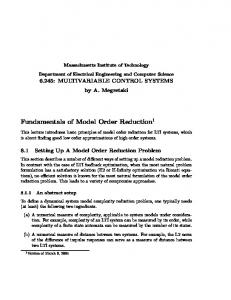
Next, we will discuss the second choice of the snapshot space. For a coarse edge Ei , we can define a oversampling domain ωi+ ⊃ Ei with ωi+ is an union of the fine-grid element, that is, ωi+ = ∪F ∈I K for some I ⊂ Th . We will show an illustration of the oversampling domain in figure 5.1.

ω +i

ωi Ei

Figure 3: An illustration of the oversampling domain (i),+

We find (ψj

(i),+

, qj

) by solving the following problem on the oversampling domain ωi+ (i),+

K −1 ψj

(i),+

+ ∇qj

∇·

(i),+ (ψj )

13

=0 =

(i) βj

in ωi+ in ωi+

(i)

(i),+

(i)

·n∂ω+ = rj for 1 ≤ j ≤ Ji+ where rj is a piecewise constant i R (i) ∂ωi+ rj (i) + with respect to the fine-grid on ∂ωi with Gaussian random value and βj = . The |ωi+ | (i) snapshot basis function ψj is then the solution of the local problem (33) with boundary condition with boundary condition ψj

(i)

ψj · n∂ωi (i) ψj

=0

· nEi

=

on ∂ωi

(i),+ ψj

· nEi

in Ei .

(i)

Similarly, the local snapshot space Vsnap is defined as the span of the snapshot basis function (i) (i) ψj and the snapshot space Vsnap is defined as the sum of the local snapshot space Vsnap . Multiscale space In this section, we will discuss the construction of the multiscale space Vms . Following the framework of [17], we will perform a dimension reduction on the snapshot space by using some local spectral problems. The spectral problems are used to select some dominant (i) modes from the local snapshot spaces Vsnap . These local dominant modes span the local multiscale space and the multiscale is the sum of these local multiscale space. For each (i) (i) (i) coarse edge Ei , we will solve a local spectral problem which find (φj , λj ) ∈ Vsnap × R such that (i)

(i)

(i)

(i) a(i) (φj , v) = λj s(i) (φj , v) ∀v ∈ Vsnap ,

where a(i) (·, ·) and s(i) (·, ·) are two symmetric positive definite bilinear forms. There are several choices for the local spectral problem. In [17, 12], authors suggested different spectral problem. In this paper, we will select one of these spectral problems. We consider the (i) (i) (i) (i) bilinear forms a(i) : Vsnap × Vsnap → R and s(i) : Vsnap × Vsnap → R are defined as a(i) (u, v) =

−1 Ei k (u · nEi )(v · nEi )

R

s(i) (u, v) =

and

R

−1 ωi k u · v +

R

ωi (∇

· u)(∇ · v) .

We assume the eigenvalue are arranged in ascending order, that is, (i)

(i)

(i)

0 < λ1 ≤ λ2 ≤ λ3 ≤ · · · . (i)

We will use the first Li eigenfunctions to span our local multiscale space Vms , namely, (i)

(i) Vms = span{φj | 1 ≤ j ≤ Lj }, (i)

where Li is the dimension of the local multsicale space Vms . The multiscale space Vms is (i) then defined as the sum of the local multiscale space Vms , that is, (i) Vms = ⊕i Vms ,

14

P and the total dimension of Vms is the sum of Li , namely, dim(Vms ) = i Li . In practice, we normally use a small number of basis functions. There are two ways to determine how many basis functions are required. One is using the eigenvalue to estimate the number of basis (i) functions Li . Following the analysis in [17], the approximation error of the multsicale space (i) (i) is related to the minimum of the eigenvalue λLi +1 . If mini {λLi +1 } is small, the multiscale space may give an inaccurate approximation of the solution. Therefore, we will need to use (i) sufficiently many multiscale basis functions to ensure min{λLi +1 } does not closed to zero. Another way to determine the number Li is using a posteriori error estimate to locate which region requires more basis functions. We can apply this approach in both the offline stage and the online stage. In the offline stage, we can solve a number of sample problems in a short time period and use the numerical result to preform the posteriori error estimate. In the online stage, we can use the online numerical result to modify the number of basis functions we used.

5.2

Adaptive approach

In this section, we will present an adaptive griding approach to construct a finite element space which gives a good approximation for the saturations and the pressure. We will determent the fine grid region Ωh by using a coarse grid indicator. There are different choices for the indicator. One of the indicators is describe in subsection 4.2. In this subsection, we introduce a residual based indicator to locate the fine grid region. We will use a fine grid finite element space in the region with large residual. That is Ωh = ∪{K ∈ TH | kRK k > θ(max{kRK k})}, K

where the residual operator Rα is defined as   ∂ RK,α = (φNα (Sw,ms , Sg,ms , Po,ms )) + ∇ · Fα,ms − qα , w ∂t Ω and the residual norm is defined as kRK k = max{ α

|Rα (w)| }. w∈Wh (K) kwkL2 (K) sup

where (Sα,ms , Po,ms , Fα,ms ) is the solution of the problem (20) in coarse grid space. We remark that these residual operators can also be used to construct online multiscale basis functions to enrich the coarse grid space.

6

Numerical Results

In this section, we present numerical experiments for the adaptive homogenization and generalized multiscale approaches using an augmented dataset from the 10th SPE comparative project [15]. Figure 4 shows the spatial distribution of x and y direction, diagonal components of the absolute permeability tensor. The reservoir domain is 120ft×30ft with coarse and fine scale grid discretizations of 22×6 and 220×60, respectively. The coarse and 15

fine grid elements are consequently 5ft×5ft and 0.5ft×0.5ft. Although not restrictive, the reservoir porosity is assumed to be homogeneous with a value of 0.2. Fine Permeability Distribution (y-direction) 4

4

2

2

x

x

Fine Permeability Distribution (x-direction)

0

0

y

y

Figure 4: Permeability distribution (log10 scale) from layer 20 of the SPE10 dataset.

The gas phase is assumed to be fully compressible with slightly compressible description for the oil and water phases described by equations, ρg = cg Pg , ρo = ρ0o expco Po ,

(34)

ρw = ρ0w expcw Pw . Here, the gas, oil, and water phase compressibility is taken to be cg = 4.7× 10− 3, co = 1×10−4 , and cw = 1×10−6 psi−1 , respectively. Further, the oil and water phase density at the standard conditions are ρ0o = 56.0 and ρ0w = 66.5 lbs/cuft, respectively. The fluid viscosities are assumed to be constant at µg = 0.018, µo = 2, and µw = 1 cP for the gas, oil, and water phases, respectively. The phase relative permeabilities are represented using Brooks Corey model as follows,  ng Sg − Sgr krg (Sg ) = krg,max , 1 − Sgr − Sor − Swr  no So − Sor (35) kro (So ) = kro,max , 1 − Sgr − Sor − Swr nw  Sw − Swr krw (Sw ) = krw,max , 1 − Sgr − Sor − Swr with endpoints krg,max = 0.6, kro,max = 0.7, krw,max = 0.8, Sgr = 0.1, Sor = 0.15, Swr = 0.2, and model exponents ng = 1.5, no = 1.2, nw = 2.0. Additionally, the gas-oil (Pcgo ) and oil-water (Pcow ) capillary pressures are also assumed to follow the Brook-Corey relationship, 1 − Sor So − Sor

λgo

1 − Swr Sw − Swr

λow

 Pcgo = Ptg  Pcow = Pto

, (36) .

Here, the entry pressures for the gas and water phases are Ptg = 5 psi and Pto = 10 psi, respectively. The model exponents are taken to be λgo = 0.5 and λow = 0.25. Figure 5 shows 16

the phase relative permeabilities and capillary pressures obtained using the aforementioned Brooks-Corey model parameters. Brooks Corey Relative Permeabilities

1

k

P

rg

cgo

k ro

0.8

Brooks Corey Capillary Pressures

100

Pcow

80

Pcgo,Pcow

k r(g,o,w)

k rw

0.6 0.4 0.2 0

60 40 20

0

0.2

0.4

0.6

0.8

0

1

0

0.2

S(g,o,w)

0.4

0.6

0.8

1

S(o,w)

Figure 5: Brooks-Corey relative permeability and capillary pressure curves.

The solution gas Rg is assumed to be a monotonic function of pressure described by, Rg (Po ) = 1 − exp−β(Po −Pd ) .

(37)

Here, β = 5×10−4 and Pd = 1000 psi is the dew point pressure. Figure 6 shows the variation of solution gas as a function of pressure. Solution Gas (Rg)

1 0.8

Rg

0.6 0.4 0.2 0 1000

1500

2000

2500

3000

3500

4000

Pressure (psi)

Figure 6: Solution gas Rg variation with pressure.

The initial conditions for the pressure and saturations are taken to be Po0 = 2500 psi, = 0.2, and So0 = 0.55. We employ a pressure and water flux (uw · n) specified boundary conditions at the top right and bottom left corners of the computational domain to mimic pressure specified production at 2500 psi and water rate specified injection wells 1 STB/day. A no flow condition is assumed on the rest of the reservoir domain boundary. In what Sg0

17

follows, we present a comparison of the oil, gas and water production rates and cumulative recoveries against a benchmark fine scale problem for both adaptive homogenization and multiscale basis approaches.

6.1

Adaptive Numerical Homogenization

In this subsection we present a comparison between a benchmark fine scale simulation and adaptive numerical homogenization approach. The tolerance for the adaptivity criterion for dynamic mesh refinement, described in subsection 4.2, is adap = 0.05. Figures 7, 8, and 9 compare the gas, oil, and water saturation profiles, respectively between the adaptive and fine scale simulations at time 25 and 75 days. The adaptivity criterion identifies the water saturation front as the transient region and adaptively refines this region of interest while using coarse scale effective properties away from the transient region. Sg at time 25 days

30

0.5

25

0.4

20 0.3

15 0.2

10 0.1

5 0

0

0

10

20

30

40

50

60

70

80

90

100

110

Sg at time 75 days

30

0.5

25

0.4

20 0.3

15 0.2

10 0.1

5 0

0

0

10

20

30

40

50

60

70

80

90

100

110

Figure 7: Adaptive homogenization (left) and fine (right) scale gas saturation profiles

We note that the gas saturation front , in Figure 7 moves faster than the oil and water saturation fronts, Figures 8 and 9, owing its high phase mobility. However, identifying the water saturation front as the transient region allows us to capture the flow physics without requiring local mesh refinement (or enrichment) on a larger computational domain. Furthermore, we are also able to accurately capture the oil bank, region of high oil saturation away from the water saturation front in Figure 8, formed due to large, mobile, initial oil saturations.

18

So at time 25 days

30

1

25

0.8

20 0.6

15 0.4

10 0.2

5 0

0

0

10

20

30

40

50

60

70

80

90

100

110

So at time 75 days

30

1

25

0.8

20 0.6

15 0.4

10 0.2

5 0

0

0

10

20

30

40

50

60

70

80

90

100

110

Figure 8: Adaptive homogenization (left) and fine (right) scale oil saturation profiles

Sw at time 25 days

30

1

25

0.8

20 0.6

15 0.4

10 0.2

5 0

0

0

10

20

30

40

50

60

70

80

90

100

110

Sw at time 75 days

30

1

25

0.8

20 0.6

15 0.4

10 0.2

5 0

0

0

10

20

30

40

50

60

70

80

90

100

110

Figure 9: Adaptive homogenization (left) and fine (right) scale water saturation profiles

Figure 10 shows a comparison between adaptive and fine scale simulations for the gas, oil, and water rates and cumulative recoveries at the production well. Production Rate (STB/day)

1

0.8

0.6

Gas (adap) Oil (adap) Water (adap) Gas (fine) Oil (fine) Water (fine)

60 50

STB

Rate (STB/day)

Cumulative Production (STB)

70 Gas (adap) Oil (adap) Water (adap) Gas (fine) Oil (fine) Water (fine)

0.4

40 30 20

0.2 10 0

0

10

20

30

40

50

60

70

80

90

0

100

Time (days)

0

10

20

30

40

50

60

70

80

90

100

Time (days)

Figure 10: Gas, oil, and water rates and cumulative recoveries at the production well for fine scale and adaptive homogenization.

19

The results show that the adaptive homogenization approach is in good agreement with the benchmark fine scale simulations for the given reservoir properties and model parameters.

6.2

Generalized mixed multiscale method

In this subsection, we will present a numerical result of the generalized mixed multiscale method for black oil equation. We will use the adaptivity criterion described in 5.2 with θ = .04. In Figure 13, 12 , 11, we will show the snapshots of the gas, oil and water saturation for both multiscale solution and the fine grid reference solution at time 25 days and 75 days. We can see that even we are using coarse grid in most of the regions, we still obtain a good coarse grid approximation of the reference solution. Sg at time 25 days

Sg at time 25 days

30

0.5

30

0.5

25

0.4

25

0.4

20

20 0.3

0.3

15

15 0.2

0.2

10

10

5 0 0

20

40

Sg at time

7560 days

80

0.1

5

0

0

100

0.1

0

0

20

40

Sg at time

7560 days

80

100

30

0.5

30

0.5

25

0.4

25

0.4

20

20 0.3

0.3

15

15 0.2

0.2

10

10

5

0.1

5

0

0

0

0

20

40

60

80

100

0.1

0

0

20

40

60

80

100

Figure 11: Generalized multiscale (left) and fine (right) scale gas saturation profiles

We observe that the fine grid refinement is mostly concentrated at the front of the water saturation front since the mass transfer in the water phase is the dominating part in the total mass transfer. In most of the regions, we are still using coarse grid piesewise constant basis functions. The adaptive approach keeps the problem size small to increase the computational speed. To improve the accuracy, we can either enriching multiscale basis function to the coarse grid space, instead of using piecewise constant function only, or using smaller adaptive tolerance. Using enriching multiscale basis function gives a better global approximation for the pressure and velocity. Using smaller adaptive tolerance can give us a finer resolution for the saturations, the pressure and the velocity locally.

20

So at time 25 days

So at time 25 days

30

1

30

1

25

0.8

25

0.8

20

20 0.6

0.6

15

15 0.4

0.4

10

10

5 0 0

20

40

So at time 7560 days

80

0.2

5

0

0

100

0.2

0

0

20

40

So at time 7560 days

80

100

30

1

30

1

25

0.8

25

0.8

20

20 0.6

0.6

15

15 0.4

0.4

10

10

5 0 0

20

40

60

80

0.2

5

0

0

100

0.2

0

0

20

40

60

80

100

Figure 12: Generalized multiscale (left) and fine (right) scale oil saturation profiles

Sw at time 25 days

Sw at time 25 days

30

1

30

1

25

0.8

25

0.8

20

20 0.6

0.6

15

15 0.4

0.4

10

10

5 0 0

20

40

Sw at time

60 days 75

80

0.2

5

0

0

100

0.2

0

0

20

40

Sw at time

60 days 75

80

100

30

1

30

1

25

0.8

25

0.8

20

20 0.6

0.6

15

15 0.4

0.4

10

10

5

0.2

5

0

0

0

0

20

40

60

80

100

0.2

0

0

20

40

60

80

100

Figure 13: Generalized multiscale (left) and fine (right) scale water saturation profiles

In Figure 14, we show show a comparison between adaptive and fine scale simulations for the gas, oil, and water rates and cumulative recoveries at the production well. We can notice that the production rate for the multiscale method is close to the reference production rate. The production curve is a little bit smoother that the reference production curve due to the coarse grid effect. Looking at the cumulative production, we find two curves are nearly the same. Production Rate (STB/day)

Cumulative Production (STB) 70

0.9

Gas(MS) Oil (MS) Water (MS) Gas(fine) Oil (fine) Water (fine)

0.8

60

50

0.6

0.5

STB

Rate (STB\day)

0.7

Gas(MS) Oil (MS) Water (MS) Gas(fine) Oil (fine) Water (fine)

0.4

40

30

0.3 20 0.2 10 0.1

0

0 0

10

20

30

40

50

60

70

80

90

100

0

Time (days)

10

20

30

40

50

60

70

80

90

100

Time (days)

Figure 14: Gas, oil, and water rates and cumulative recoveries at the production well for fine scale and generalized multiscale.

21

7

Summary

We presented two approaches for model order reduction namely: (1) the adaptive numerical homogenization and (2) the generalized multiscale basis functions. An expanded mixed variational formulation is used by both approaches to separate scale of the flow and transport problems. The adaptive numerical homogenization approach performs local numerical homogenization to pre-compute effective properties (permeability, porosity, relative permeability, and capillary pressure) and dynamic mesh refinement to fine scale during simulation runtime based upon an adaptivity criterion. On the other hand, the generalized multiscale basis functions approach construct a multiscale velocity basis functions as an offline (or precompute) step. We describe a benchmark fine scale, black oil model problem to compare the accuracy of each of these two approaches. The numerical results indicate that both approaches accurately capture the multiphase flow physics while reducing the problem size compared to the benchmark fine scale simulation. This benchmark study enables us to rigorously assess, in the near future, the computational efficiencies required of each of the aforementioned model order reduction techniques.

References [1] Jorg E Aarnes. On the use of a mixed multiscale finite element method for greaterflexibility and increased speed or improved accuracy in reservoir simulation. Multiscale Modeling & Simulation, 2(3):421–439, 2004. [2] Jørg E Aarnes and Yalchin Efendiev. An adaptive multiscale method for simulation of fluid flow in heterogeneous porous media. Multiscale Modeling & Simulation, 5(3):918– 939, 2006. [3] Gr´egoire Allaire. Homogenization and two-scale convergence. SIAM Journal on Mathematical Analysis, 23(6):1482–1518, 1992. [4] Yerlan Amanbek, Gurpreet Singh, Mary F. Wheeler, and Hans van Duijn. Adaptive numerical homogenization for upscaling single phase flow and transport. ICES Report, 12(17), 2017. [5] B. Amaziane, S. Antontsev, L. Pankratov, and A. Piatnitski. Homogenization of immiscible compressible two-phase flow in porous media: Application to gas migration in a nuclear waste repository. Multiscale Modeling & Simulation, 8(5):2023–2047, 2010. [6] Brahim Amaziane, S Antontsev, Leonid Pankratov, and Andrey Piatnitski. Homogenization of immiscible compressible two-phase flow in porous media: application to gas migration in a nuclear waste repository. Multiscale Modeling & Simulation, 8(5):2023– 2047, 2010. [7] Brahim Amaziane, Alain Bourgeat, and Mladen Jurak. Effective macrodiffusion in solute transport through heterogeneous porous media. Multiscale Modeling & Simulation, 5(1):184–204, 2006.

22

[8] Brahim Amaziane, Leonid Pankratov, and Andrey Piatnitski. Homogenization of immiscible compressible two-phase flow in highly heterogeneous porous media with discontinuous capillary pressures. Mathematical Models and Methods in Applied Sciences, 24(07):1421–1451, 2014. [9] Todd Arbogast, Gergina Pencheva, Mary F Wheeler, and Ivan Yotov. A multiscale mortar mixed finite element method. Multiscale Modeling & Simulation, 6(1):319–346, 2007. [10] Alain Bensoussan, Jacques-Louis Lions, and George Papanicolaou. Asymptotic analysis for periodic structures, volume 5. North-Holland Publishing Company Amsterdam, 1978. [11] Alain Bourgeat. Homogenized behavior of two-phase flows in naturally fractured reservoirs with uniform fractures distribution. Computer Methods in Applied Mechanics and Engineering, 47(1-2):205–216, 1984. [12] Ho Yuen Chan, Eric Chung, and Yalchin Efendiev. Adaptive mixed gmsfem for flows in heterogeneous media. Numerical Mathematics: Theory, Methods and Applications, 9(4):497–527, 2016. [13] Y Chen, Louis J Durlofsky, M Gerritsen, and Xian-Huan Wen. A coupled local–global upscaling approach for simulating flow in highly heterogeneous formations. Advances in Water Resources, 26(10):1041–1060, 2003. [14] Zhiming Chen and Thomas Hou. A mixed multiscale finite element method for elliptic problems with oscillating coefficients. Mathematics of Computation, 72(242):541–576, 2003. [15] M. A. Christie and M. J. Blunt. Tenth spe comparative solution project: A comparison of upscaling techniques. SPE Reservoir Evaluation and Engineering, 4(04), 2001. [16] Eric Chung, Yalchin Efendiev, and Thomas Y Hou. Adaptive multiscale model reduction with generalized multiscale finite element methods. Journal of Computational Physics, 320:69–95, 2016. [17] Eric T Chung, Yalchin Efendiev, and Chak Shing Lee. Mixed generalized multiscale finite element methods and applications. Multiscale Modeling & Simulation, 13(1):338– 366, 2015. [18] Eric T Chung, Wing Tat Leung, Maria Vasilyeva, and Yating Wang. Multiscale model reduction for transport and flow problems in perforated domains. Journal of Computational and Applied Mathematics, 330:519–535, 2018. [19] Louis J Durlofsky. Numerical calculation of equivalent grid block permeability tensors for heterogeneous porous media. Water resources research, 27(5):699–708, 1991. [20] Yalchin Efendiev, Juan Galvis, and Thomas Y Hou. Generalized multiscale finite element methods (gmsfem). Journal of Computational Physics, 251:116–135, 2013. 23

[21] Thomas Y Hou and Xiao-Hui Wu. A multiscale finite element method for elliptic problems in composite materials and porous media. Journal of computational physics, 134(1):169–189, 1997. [22] Patrick Jenny, SH Lee, and Hamdi A Tchelepi. Multi-scale finite-volume method for elliptic problems in subsurface flow simulation. Journal of Computational Physics, 187(1):47–67, 2003. [23] Vasilii Vasil’evich Jikov, Sergei M Kozlov, and Olga Arsen’evna Oleinik. Homogenization of differential operators and integral functionals. Springer Science & Business Media, 2012. [24] Andro Mikeli´c, Vincent Devigne, and CJ Van Duijn. Rigorous upscaling of the reactive flow through a pore, under dominant peclet and damkohler numbers. SIAM journal on mathematical analysis, 38(4):1262–1287, 2006. [25] Reza Tavakoli, Hongkyu Yoon, Mojdeh Delshad, Ahmed H. ElSheikh, Mary F. Wheeler, and Bill W. Arnold. Comparison of ensemble filtering algorithms and nullspace monte carlo for parameter estimation and uncertainty quantification using co2 sequestration data. Water Resources Research, 49(12):8108–8127, 2013. [26] Sunil G Thomas and Mary F Wheeler. Enhanced velocity mixed finite element methods for modeling coupled flow and transport on non-matching multiblock grids. Computational Geosciences, 15(4):605–625, 2011. [27] John A Wheeler, Mary F Wheeler, and Ivan Yotov. Enhanced velocity mixed finite element methods for flow in multiblock domains. Computational Geosciences, 6(34):315–332, 2002. [28] Xiao-Hui Wu, Y Efendiev, and Thomas Y Hou. Analysis of upscaling absolute permeability. Discrete and Continuous Dynamical Systems Series B, 2(2):185–204, 2002.

24