Model Predictive Control Approach to Online Computation of Demand-Side Flexibility of Commercial Buildings HVAC Systems for Supply Following
Mehdi Maasoumy†, Catherine Rosenberg♦ , Alberto Sangiovanni-Vincentelli∗, Duncan S. Callaway△
Abstract— Commercial buildings have inherent flexibility in how their HVAC systems consume electricity. We investigate how to take advantage of this flexibility. We first propose a means to define and quantify the flexibility of a commercial building. We then propose a contractual framework that could be used by the building operator and the utility to declare flexibility on the one side and reward structure on the other side. We then design a control mechanism for the building to decide its flexibility for the next contractual period to maximize the reward, given the contractual framework. Finally, we perform at-scale experiments to demonstrate the feasibility of the proposed algorithm.
is controlled. In this paper, we identify and quantify “flexibility”. Then, a contractual framework between the utility and the building operator is designed so that the building can “declare” its flexibility and be rewarded for it. Finally, a control algorithm is proposed that allows the operation of building under this framework and at-scale experiments are carried out to demonstrate the high potential of commercial buildings as a source of flexibility, and the feasibility of the developed algorithm.
I. I NTRODUCTION
We focus on commercial buildings due to the following reasons: 1) Commercial buildings account for more than 35% of electricity consumption in the US. 2) More than 30% of commercial buildings have adopted Building Energy Management System (BEMS) technology which facilitate the communication with the grid system operators for providing flexibility. The majority of these buildings are also equipped with variable frequency drives, which in coordination with BEMS, can modulate the heating, ventilation and air conditioning (HVAC) system power consumption frequently (in the order of seconds). 3) Compared to a typical residential building, commercial buildings typically have larger HVAC systems and therefore consume more electricity. About 15% of electricity consumption in commercial buildings is related to the fans of HVAC systems. Fans are the main drivers to move the conditioned air from the air handling units (AHU) to the rooms for climate control. For instance, the main supply fans that feed Sutardja Dai Hall on UC Berkeley campus can spin at variable speeds, with the corresponding power consumption which is proportional to the cube of fan speed, with the maximum rated power of 134 KW or about 14% of the maximum power consumed in that building. Moreover, we can directly control their power, upward or downward making it an ideal candidate for ancillary demand-response. See [1]–[5] for more information about the physics and control of HVAC systems.
Consumers of energy usually do not pay attention to when they use energy. Demand for electricity tends to rise specially at times when it seems natural to use it; So natural in fact that we all tend to use it at the same time and in similar ways. On days when demand for electricity is high, extra power plants are needed to meet the demand. There are environmentally-friendly alternatives to adding more generation. Electricity customers can voluntarily trim their electricity use during peak periods or choose to use electricity at a less congested time, a strategy called “SupplyFollowing” (SF). With SF programs, utilities provide incentives to encourage consumers to reduce their demand during peak periods. Smart grids are enabling the transformation from a demand-following strategy to a supply-following one. Smart buildings are essential elements of the smart grid and can play a significant role in its operation. A building has some inherent flexibility in the way its HVAC system consumes electricity while respecting the comfort of its occupants. This flexibility could be used to reduce costs if the electricity price is time-varying, or could be traded (i.e., sold to the utility) if a proper contractual framework exists. Typically the electricity consumption of a commercial building is controlled by a process that aims at reducing costs. Among the many possible ways to design such a process, Model Predictive Control (MPC) stands out. In order to use the potential of commercial buildings as providers of flexibility to the smart grid, we need to fundamentally redesign the way a building, and in particular its HVAC, † Department of Mechanical Engineering, University of California, Berkeley, CA 94720, USA. Corresponding author. Email:
[email protected] ♦ Department of Electrical and Computer Engineering, University of Waterloo, Canada. ∗ Department of Electrical Engineering and Computer Sciences, University of California, Berkeley, CA 94720, USA. △ Energy and Resources Group, University of California, Berkeley, CA 94720, USA.
II. BASELINE S YSTEM
AND
C ONTRACT
A. The Baseline System We consider a commercial building that has an HVAC system controlled by an MPC as our baseline. The MPC has the objective of minimizing the total energy cost (in dollar value). Let the time be slotted with τ as the length of each time slot, and let H m be the prediction horizon (in number of time-slots) of the MPC. System dynamics is also discretized with a sampling time of τ . Typical values for τ and H m range from 15 min to 1 hr for τ and a
few hours to a few days, e.g., 3 to 72 time slots (with the assumption of 1 hr for each time slot) for H m . The choice of H m depends on how far in the future the estimation of the predicted values have an acceptable accuracy, and also on how far in the future the required information (e.g. cost of energy) is available. In this paper we use τ = 1 hr and H m = 24 hrs. At each time t, the predictive controller solves the following optimal control problem to compute the optimal vector ~ut = [ut , . . . , ut+H m −1 ], where ut+k is the air mass flow to the thermal zones of the building. The inputs to the optimal control problem are the states (i.e. zone temperatures) xt (as initial condition), the e set of electric energy prices {πte , . . . , πt+H m −1 }, the nonelectric and non-fan energy prices, such as gas price for heating π ne,h , and cooling π ne,c which are considered timeinvariant, a set of constraints Xt+k on the system states of the type: ”xt+k should be in Xt+k for all times t + k where k ∈ {1, . . . , H m })”, a set of constraints Ut+k on system inputs for all k ∈ {0, . . . , H m − 1}, and an estimate on unmodelled disturbances dt+k (e.g., outside temperature or building occupancy [6]) for all k ∈ {0, . . . , H m − 1} for the next H m time slots. The optimization problem is as follows: m HX −1 e out min Chvac (ut+k , πt+k , π ne,c , π ne,h , Tt+k ) (1) u ~t
s.t.
k=0
xt+k+1 = f (xt+k , ut+k , dt+k ), k = 0, ..., H m − 1 xt+k ∈ Xt+k , k = 1, ..., H m k = 0, ..., H m − 1
ut+k ∈ Ut+k ,
where T out is the outside air temperature, f captures the system dynamics, and the total HVAC power consumption cost Chvac (t) is the summation of fan power, cooling power and heating power, given by: Chvac (t) = π e (t)Pf (t) + π ne,c Pc (t) + π ne,h Ph (t) (2) where with the assumption of no recirculation of air, and without loss of generality, these power consumptions for time slot [t, t + 1] (with the assumptions of constant air mass flow and price of energy over [t, t + 1]) are calculated as follows: Pf (ut ) = c1 .u3t + c2 .u2t + c3 .ut + c4 Ph (ut , Ttout ) Pc (ut , Ttout )
= =
s
cp .ut .(T − Ttout )/COPh cp .ut .(Ttout − T s )/COPc
(3) (4) (5)
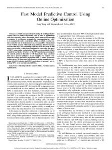
where c1 , c2 , c3 , and c4 are constants of the fan as shown in Fig. 1, cp is the specific heat of air, and COPh , and COPc are the coefficients of performance for the heating system and the cooling system, respectively, and the supply air temperature T s is considered constant. To move the coolant fluid around, heating and cooling systems use pumps which consume electric power. However, we assume that electric power consumption of pumps is negligible compared to the non-electric heating and cooling powers of these systems. (see [3], [4] for more details). Hence, the MPC solution to (1) is an optimal air mass flow trajectory (also called an air mass flow profile) ~u∗t = [u∗t , . . . , u∗t+H m −1 ]. Only the first entry of ~u∗t is implemented at time t. At the next time step, t + 1, the horizon of MPC
Fig. 1. Fan power consumption versus volume flow rate. Data is for January through August of 2013.
is receded by one step, a new MPC is set up, and solved to obtain ~u∗t+1 = [u∗t+1 , . . . , u∗t+H m ]. Again, the first entry is implemented on the system, and the horizon is receded, and this process repeats until the whole time frame of interest is covered. At each time t, the optimal air mass flow vector for the next H time steps is given by ~u∗t = [u∗t , . . . , u∗t+H m −1 ], with corresponding fan power flow profile of Pf (~u∗ ) = [Pf (u∗t ), . . . , Pf (u∗t+H m −1 )]. In the following, we will omit the reference to t in the profile and define a power profile as a vector Pf (~u∗ ) = [Pf (u∗0 ), . . . , Pf (u∗H m −1 )]. B. The Baseline Contract The baseline contract corresponding to this baseline system is very simple. Namely, the building can consume what it wants at all times and it pays πte per unit of consumed electricity at P time t (i.e., if the time span is of duration ∆, t+∆ e then it pays k=t π (k)Pf (k) for electric power). Hence, the only information being exchanged between the utility e and the BM is the real-time price vector [π0e , . . . , πH m −1 ] in ($/kWh) sent by the utility to the building (π ne,c and π ne,h are considered constant and known). Then the building solves the MPC (1) to compute what its electricity consumption profile/trajectory would be in the next H m time slots. As described, this MPC would minimize its total cost in the next H m time slots while respecting the building and the occupants (comfort) constraints. Let ~u∗ denote the trajectory that is the solution to this MPC and let C(~u∗ ) be its cost. III. F LEXIBILITY, C ONTRACTUAL F RAMEWORK C ONTROL A LGORITHM
AND
A. Definition of Flexibility We define flexibility in terms of two envelope air mass flow profiles e~l = [eltcs , . . . , eltce ] a lower envelope, and e~u = [eutcs , . . . , eutce ] an upper envelope. tcs and tce are contract start and end times. Based on the requirement from the utility that flexibility of each building has to be determined ahead of time we pick tcs , and consequently tcs as follows: tcs ≥ 1 (6) m tcs + 1 ≤ tce ≪ H − 1 (7) tce − tcs = H c
(8)
where H c is the length of the contract. Typical values for H c are much smaller than H m , and can take values from one slot to a few time slots. The BEMS computes e~l =
TABLE I N OMENCLATURE Parameter τ Hm Hc dt Ttout Ts Xt Ut πte π ne,c π ne,h COPh COPc tcs tce {β t , β t } Variable xt ut wt eu k elk {ϕt , ϕt } {ψ t , ψt } Chvac (ut , πte ) Pf , Ph , Pc R(Φ, B)
Definition Sampling time for discretizing continuous system dynamics Prediction horizon of MPC Horizon (length) of the proposed contract Disturbance to the system at time t which comprises outside temperature, occupancy, solar radiation, etc. Outside air temperature at time t Supply air temperature exiting air handling unit (AHU) Set of permissible states at time t Set of permissible inputs at time t Per-unit price of electric energy at time t – ($/kW h) Per-unit price of non-electric cooling energy – ($/kW h) Per-unit price of non-electric heating energy – ($/kW h) Coefficient of performance of heating system Coefficient of performance of cooling system Contract start time Contract end time Reward paid from the utility to the building at time t for providing upward flexibility (β t ),and down flexibility (β t ) – ($/kW ) Definition State of the system at time t Input to the system at time t Uncertainty variable introduced to derive the worst-case (robustified) optimal control problem Upper envelope for safe air mass flow Lower envelope for safe air mass flow Provided upward (ϕ), and downward (ϕ) flexibility by building at time t in unit of air flow Provided upward (ψ), and downward (ψ) flexibility by building at time t in unit of power Total HVAC energy consumption cost at time t Power consumption of fan, heating and cooling systems Reward from utility to building for providing flexibility
[el0 , . . . , elH m −1 ] a lower envelope and e~u = [eu0 , . . . , euH m −1 ] an upper envelope (using the algorithm described later in the paper), so that any air mass flow profile ~u = [u0 , . . . , uH m −1 ] such that for all k ∈ {0, . . . , H m − 1}, elk ≤ uk ≤ euk is feasible; i.e. no building constraints are violated at anytime. The corresponding fan power consumption envelopes are Pf (e~l ) = [Pf (el0 ), . . . , P~f (elH m −1 )] and Pf (e~u ) = [Pf (eu0 ), . . . , Pf (euH m −1 )]. However the building only declares the first H c values of the envelope as flexibility, namely, e~l = [eltcs , . . . , eltcs +H c ] a lower envelope, and e~u = [eutcs , . . . , eutcs +H c ] an upper envelope, at the beginning of each contract. The reason for declaring a subset of the obtained envelopes is that due to model mismatch, imperfect predictions of disturbance and so on, the later values in the H m -step envelopes may not be accurate and need to be updated in the next time step. By declaring these two envelopes, the building has essentially declared its flexibility for the next H c time slots. Note that there is NO objective function and energy cost here, we define flexibility with respect to feasibility criteria. By declaring these two envelopes, the building manager is telling the utility: “I allow you to select any power trajectory Pf (~u) = [Pf (utcs ), . . . , Pf (utce )] such that for all k ∈ {tcs , . . . , tce }, Pf (elk ) ≤ Pf (uk ) ≤ Pf (euk )”.
To quantify the flexibility provided at each time step k, we need to define a single metric. The metric that is natural to use is the difference between the upper and lower power envelope that can be consumed by the building without violating any constraints. Hence, Flexibility(k) , Pf (euk ) − Pf (elk )
(9)
B. Contract Framework In the proposed framework, the building operator can declare its flexibility contract to the utility. The flexibility declared by the building operator would only be significant if the reward is appropriate. It is important to understand that by allowing the utility to select any trajectory Pf (~u) = [Pf (utcs ), . . . , Pf (utce )] or correspondingly ~u = [utcs , . . . , utce ] such that for all k ∈ {tcs , . . . , tce } elk ≤ uk ≤ euk , the building might consume more or be in a worse state at the end of the H c time slots. We define the “flexibility” contract as follows: The utility charges the building operator for its baseline power consumption Pf (~u∗ ) which is agreed upon at the time of the contract, irrespective of the deviations from the baseline power consumption due to flexibility signals from the utility, and the utility rewards the building operator for its declared flexibility. Hence, this contract is deterministic in the sense that from the beginning of the contract, the utility and the building operator both know how much money each has to pay; the building pays for consuming Pf (u∗t ) at rate πte , and the utility pays the building for providing downward flexibility at rate β t and for providing upward flexibility at rate β t . In short, the contract implementation steps are as follows: 1) The building and the utility agree upon a contract length, H c . e 2) The utility declares [π0e , . . . , πH m −1 ], as per unit price of electric energy, [β 0 , . . . , β H m −1 ] in ($/kW ), as reward for down flexibility, and [β 0 , . . . , β H m −1 ] in ($/kW ), as reward for upward flexibility. If the utility is not willing to commit to the flexibility rates for the time span beyond the next immediate contract period, i.e. [β H c +1 , . . . , β H m −1 ], and [β H c +1 , . . . , β H m −1 ], the building operator can then obtain an estimate of these values from historical data. 3) The building operator computes the baseline air mass flow u∗k and the two envelopes elk and euk , for the time frame k = 0, 1, . . . , H m − 1, with its overall cost if it uses the flexibility contract as follows: Building Operator Payment
z Cf =
m HX −1
}|
{
Chvac (uk , πke )
k=0 m HX −1
−
(10)
β k ψ(uk , elk )
−
β k ψ(uk , euk )
k=1
k=1
|
m HX −1
{z
Reward for Providing Flexibility
}
where ψ, and ψ are defined as: ψ(uk , euk ) , Pf (euk ) − Pf (uk )
(11a)
ψ(uk , elk )
(11b)
, Pf (uk ) −
Pf (elk )
4) The building operator then declares Pf (e~l ) and Pf (e~u ), the baseline profile Pf (~u∗ ) that it will consume and the length of the contract H c to the utility. 5) In the next H c time slots, the utility will send signals (sk )’s, such that Pf (elk ) ≤ sk ≤ Pf (euk ) and the building operator has to obey the signals, i.e., has to consume power in time slot k equal to sk . Flexibility signal sk may arrive as frequently as every few seconds, as mentioned earlier.
2) Putting It All Together: We assume at each time step t, that the current state of the building is known. Furthermore, the prediction of the outside temperature, inside heat generation, and constraints on the system states and inputs are known. The outputs of the algorithm is the nominal power consumption of the building, u∗t+k for k ∈ {0, ..., H m − 1}, the flexibility that the building can provide, Φ∗t+k+1 for k ∈ {0, ..., H m − 1}, for future time steps, without violating constraints. Based on this set of information, the BEMS can decide how much flexibility to offer. It may declare very small flexibility and hence get a cost close to Chvac . The algorithm described above can be formulated as a minmax MPC problem. At time t we are interested in solving the following robust optimal control problem:
C. Proposed Control Mechanism As discussed in Section III-B, if the utility provides a e vector ~π e = [π0e , . . . , πH m −1 ] of per-unit of energy prices per time P slot,mthen BEMS could try to minimize its total energy H −1 cost k=0 Chvac (uk , πk , Tkout ). In that case, BEMS uses building flexibility selfishly to minimize its cost. Hence, BEMS does value (and does use) its flexibility. If the utility values the flexibility that the building HVAC system can offer, it has to provide the right incentive and the right mechanism to declare this flexibility. 1) Formalizing Flexibility and Incentive in the MPC Framework: We say that the building can offer a flexibility ~ in fan power or equivalently a flexibility Φ := ~ ψ} Ψ := {ψ, {~ ϕ, ~ϕ} in air mass flow which comprises down flexibility, ~ from the contract start time ϕ, and upward flexibility ϕ, ~ tcs = t + 1 to the contract end time tce := t + 1 + H c for 1 ≤ H c ≤ H m time slots (starting from x0 ) if there exist two trajectories e~l = ~u + ~ ϕ and e~u = ~u + ~ϕ, that satisfy: ϕk ≤ 0,
ϕk ≥ 0
∀k ∈ {tcs , . . . , tce }
(12)
f (xk , uk + ϕk , dk ) ∈ Xk+1
∀k + 1 ∈ {tcs , . . . , tce } (13)
f (xk , uk + ϕk , dk ) ∈ Xk+1 uk + ϕk ∈ Uk
∀k + 1 ∈ {tcs , . . . , tce } (14) ∀k ∈ {tcs , . . . , tce } (15)
uk + ϕk ∈ Uk
∀k ∈ {tcs , . . . , tce }
(16)
What we defined here is a flexibility over multiple time ~ (i.e., the utility slots. Assume that BEMS declares ~ ϕ and ϕ might choose any fan power (and consequently air flow u ˆk ) in time step tcs ≤ k ≤ tce as long as u∗k + ϕk ≤ u ˆk ≤ u∗k + ϕk ), where u∗k is the baseline air mass flow. Hence, we “center” the flexibility around u∗ . The flexibility-aware optimal control problem should minimize the cost function which is composed of the cost for the baseline HVAC power consumption, Chvac , (i.e., the cost of problem (1)), minus the reward for the flexibility, R, which is computed as follows: T T ~ u, ϕ ~ u, ~ ~ B) ~ = ~β .ψ(~ ~ ) + ~β .ψ(~ R(Φ, ϕ)
(17)
where B~ := {~β, ~β}, and ψ(.), and ψ(.) are given by (11), in which e~l = ~u + ~ϕ and e~u = ~u + ~ϕ.
Min-max Problem min max
~ t+1 w ~t u ~ t ,Φ
m HX −1
Chvac (ut+k , πt+k ) − R(Φt+k+1 , Bt+k+1 )
k=0
(18a) subject to:
xt+k+1 = f (xt+k , ut+k + wt+k , dk ) ∀ k = 0, ..., H m − 1 ∀ wt s.t. : ϕt ≤ wt ≤ ϕt
(18b) (18c)
∀ wt+k s.t. : ϕt+k ≤ wt+k ≤ ϕt+k ∀k = 1, ..., H m − 1 ϕt+k ≥ 0, ∀ k = 1, ...H m − 1 ϕt+k ≤ 0, ∀ k = 1, ...H m − 1
(18d) (18e) (18f)
xt+k ∈ Xt+k ∀ k = 1, ..., H m (18g) ut+k + wt+k ∈ Ut+k ∀ k = 0, ..., H m−1 (18h)
Note that ϕt and ϕt are computed in the previous time step and are constant values in this formulation, while ϕt+k and ϕt+k for k ∈ {1, . . . , H m −1} are optimization variables and will be computed in the current time step by solving the optimal control problem (18). The inner maximization problem robustifies the optimization problem and derives the worst-case scenario cost and constraints. The outer minimization problem solves for its ~ t+1 ) while it is guaranteed that the conarguments (~ut , Φ straints are satisfied for all values of uncertainty w, as long as it is within the range ϕt+k ≤ wt+k ≤ ϕt+k for k ∈ {1, . . . , H m − 1}. Theorem [7]: Let C be a closed convex set and let f : C → R be a convex function. Then if f attains a maximum over C, it attains a maximum at some extreme point of C. According to the theorem above, the analytic worst-case solution can be obtained. Closed convex sets can be characterized as the intersections of closed half-spaces (i.e. sets of points in space that lie on and to one side of a hyperplane). The feasible set for states, i.e. the temperature of the rooms in the building and inputs, i.e. air mass flow into the thermal
Fig. 2. Schematic of the proposed architecture for contractual framework.
zones, are defined by: Xk := {x | T k ≤ x ≤ T k }
(19)
Uk := {u | U k ≤ u ≤ U k }
(20)
where T k , and T k are the upper and lower temperature limits and U k , and U k are the upper and lower feasible air mass flow at time t. Therefore, the feasible set of (18) is closed and convex. The objective function is also convex on w, as the max is over variable w. In fact, w does not appear in the cost function. The objective function is a linear function on w and hence it is concave. We also consider a linearized state update equation as follows: xt+1 = Axt + But + Edt
(21)
the nonlinear system dynamics has been linearized with the forward Euler integration formula with time-step τ = 1 hr. Hence, the min-max problem (18) is equivalent to: Minimization Problem min
~ t+1 u t ,Φ ~
s. t.:
m HX −1
Chvac (ut+k , πt+k ) − R(Φt+k+1 , Bt+k+1 )
k=0
xt+k+1 = f (xt+k , ut+k + ϕt+k , dt+k ) ∀k = 0, ..., H m − 1 xt+k+1 = f (xt+k , ut+k + ϕt+k , dt+k ) ∀k = 0, ..., H m − 1 ϕt+k ≥ 0, ∀ k = 1, ...H m − 1 ϕt+k ≤ 0, ∀ k = 1, ...H m − 1
(22a) (22b) (22c) (22d) (22e)
(22f) xt+k ∈ Xt+k ∀ k = 1, ..., H m xt+k ∈ Xt+k ∀ k = 1, ..., H m (22g) ut+k + ϕt+k ∈ Ut+k ∀ k = 0, ..., H m − 1 (22h) ut+k + ϕt+k ∈ Ut+k ∀ k = 0, ..., H m − 1 (22i)
The argmin of the optimization problem (22) is the nominal power consumption, u∗t+k , and the maximum available flexibility, Φ∗t+k , ∀ k = 0, ..., H m − 1. The building declares u∗t+k , and Φ∗t+1+k for the time slots: ∀ k = 0, ..., H c − 1 to the utility. After H c time slots, the BEMS collects the
updated parameters such as new measurements and disturbance predictions, and sets up the new MPC algorithm for the time step k = H c , H c + 1, . . . , H c + H m − 1, and solves the new MPC for this time frame and uses only the first H c values of baseline power consumption and flexibility, i.e. for k = H c , . . . , 2H c − 1, and this process repeats. Fig. 2 shows the schematic of the entire system architecture. The solid line power flow arrows correspond to the baseline system and contract. The ancillary power flow via the flexibility contract is shown with dashed line arrow. Real-time state of the system such as occupancy, internal heat, outside weather condition, building temperature, state and input constraints are passed as input to the algorithm. The utility also communicates information such as per-unit energy and upward and downward flexibility prices to the BEMS (or effectively to the algorithm). The output of the algorithm includes baseline power consumption, downward flexibility and upward flexibility values, and cost. Within the flexibility contract framework, this information is communicated to the utility. Consequently, a flexibility signal st is sent from the utility to the building to be tracked by the HVAC fan. Essentially, the utility has control of the building consumption for the next Hc time slots. The control strategy is actuated by sending flexibility signals (similar to frequency regulation signals). These signals can be sent as frequently as every few seconds. In fact, we show through experiments on a real building in Section V, that buildings with HVAC systems equipped with variable frequency drive (VFD) fans are capable of tracking such signals very fast (e.g. within a few seconds). IV. C OMPUTATIONAL R ESULTS The algorithm presented in Section III-C was implemented on a building model developed and validated against historical data in [4], [6]. We used Yalmip [8], an interface to optimization solvers available as a MATLAB toolbox, for rapid prototyping of optimal control problems. The nonlinear optimization problem solver Ipopt [9], was used to solve the resulting nonlinear optimization problem arising from the MPC approach. We use sampling time of τ = 1 hr. We assess the performance of the algorithm for the following scenarios. Scenario I: Different reward rates have been considered for upward and downward flexibility at each time step. In particular, downward flexibility is rewarded more than upward flexibility (β > β), for most of the time. Since MPC maintains the comfort level using the least possible amount of energy, buildings that are operated under nominal MPC such as (1) have no down flexibility (for extended period of time, i.e. 1 hr or more). However we show that via proper incentives and by solving (22), it is possible to provide downward flexibility when most needed. The results of this scenario are shown in Fig. 3 for the case when ancillary signals are received from the utility every minute: no system constraint (e.g. temperature being within the comfort zone) will be violated when the fan speed enforcement is performed for arbitrary values of fan speed as long as fan power
Fig. 3. Scenario I: The Per-unit energy rate, and upward and downward flexibility reward are shown in the lowest figure. The middle figure shows the resulting flexibility at each time, and the top figure shows the resulting room temperature. Flexibility signals are sent every minute from the utility to the building.
consumption, and consequently fan speed is within the safe envelope calculated by the algorithm. It is shown in Fig. 3 that maximum flexibility (100%) is provided at times when the room temperature is far from the boundaries of the comfort zone. The flexibility decreases as the temperature of the room approaches the comfort zone boundary, and is minimum (about 0-15% in this case) when room temperature is fairly close to the boundaries of the comfort zone, and the reward for flexibility is not high enough. Scenario II: In this scenario we test the algorithm when no reward for providing flexibility is provided (i.e. β = β = 0). Results are shown in Fig. 4. In this case the MPC ”selfishly” uses the thermal capacitance of the building to minimize energy cost. This case yields to an MPC policy similar to nominal MPC (1). As expected, the resulting flexibility is very small throughout the day. Scenario III: In this case, the amount of reward to the building for upward and downward flexibility is the same as Scenario I. Furthermore, the BM is encouraged to provide equal upward and downward flexibility as long as possible. This requirement has been enforced by adding an extra penalty term to the cost function as follows: cost := cost + γtT .|ϕt − ϕt |
(23)
where γ ≫ 0 is a constant, and |.| returns the absolute value of its argument. Larger value of γ makes the equality of upward and downward flexibility to hold for a longer period. However, in this case, we lose the guaranteed maximization of the economic benefit of the building due to the newly added term in the cost function. Fig. 5 shows the result for this scenario. Maximum flexibility (100%) happens during
Fig. 4. Scenario II: In this case we consider β = β = 0. This results into a performance similar to the one of the nominal MPC (1).
unoccupied hours and when the reward for flexibility is high. In this case minimum flexibility is 0% and it happens during 6 to 7 am, 9 to 10 am, and 12 to 1 pm. The room temperature is close to the comfort-zone boundary. The per-unit price of electricity is high, and the reward for upward and downward flexibility is very small. Hence, the algorithm provides no flexibility at these time periods. In Fig. 5 the frequency of flexibility signals is 1 hr. By picking a large value for the period of flexibility signal arrivals, we show that no system constraint will be violated when the fan speed is constrained even for long time periods, as long as the fan power consumption and consequently fan speed is within the safe envelope calculated by the algorithm. V. E XPERIMENTAL R ESULTS A. Tracking Ancillary Signals by VAV-equipped Fans We ran some experiments to demonstrate that it is indeed feasible to track the flexibility signals received from utility (sk : where elk ≤ sk ≤ euk ) very fast. We run our experiments in a new building constructed four years ago (2009) on the UC Berkeley campus named Sutardja Dai Hall (SDH). It is a 141,000 square-foot modern building that houses several laboratories, including a nanofabrication lab, dozens of classrooms and collaborative work spaces. It contains a Siemens building management system called Apogee [10] which is connected to an sMAP server [11] co-located with the Apogee server. We run our experiments using a control platform built on sMAP, whereby control points are set programmatically upon approval from the building manager. The energy data of this building is stored in the cloud and is accessible to the public at [12]. The BEMS of the experiment set up is shown in Fig. 6. There are two sets of 9 fans namely AH2A and AH2B with a
Fig. 6. Building management system of the CITRIS hall, our experimental set up located on the campus of UC Berkeley.
Fig. 5. Scenario III: In this case we use the cost function presented in (23) to push the algorithm to produce equal up and downward flexibility as long as possible. Frequency of flexibility signals is 1 hr.
total capacity of 180 hp (about 134 kW). The existing control mechanism is designed to maintain the pressure in the HVAC ducts at the set point value by setting the Supply Duct Static Pressure (SDSP) setpoint. If the pressure drops below the setpoint (e.g. due to the opening of more dampers at the room level, or to the increase of the SDSP setpoint) the two sets of fans will spin faster to compensate for the change in the system and increase the pressure in the duct work to reach the setpoint. And in the case that the pressure goes above the setpoint (e.g. due to the closing of more dampers or to the decrease of the SDSP setpoint), the fan speed will decrease to bring down the pressure to the setpoint. The air handling unit (AHU) maintains an almost constant supply temperature (T s ) in the supply air duct to be sent to the rooms. If one room needs more heating, the air is reheated locally at the Variable Air Volume (VAV) box designated for each room, to increase the supply air temperature for that specific room. The flow of air to each room (m ˙ s ) is controlled by opening and closing of the dampers at the VAV level. Several experiments were conducted on this test-bed to prove our hypothesis that it is indeed feasible to track the ancillary signal sk received from the utility without affecting the comfort of the occupants. Here we report the two experiments performed on May 17 of 2013. Experiment 1 was conducted from 12:45 pm to 13:15 pm. and Experiment 2 was performed from 5:30 pm to 6:15 pm of the same day. Experiments were done by frequently changing the SDSP setpoint. SDSP is normally kept at 1.75 inch WC (inch Water Column). Due to safety reasons it is advised to always keep the duct pressure within 1.2 and 1.9 inch WC. Hence, we perform the experiments by changing the SDSP between these two values. In Experiment 1 the set
point was changed every minute to values randomly selected in the range [1.2, 1.9] and held at that value for one minute. In Experiment 2, the same procedure was done but every three minutes, and the SDSP setpoint was kept at the new value for three minutes. The results are shown in Fig. 7 and Fig. 8. In Fig. 7 we present the SDSP setpoint signal, as input of the experiment and the power consumption of the fan, as output of the experiment. It can be observed that the fan power consumption can vary up to 25% within a few seconds around its nominal power consumption at the time of the experiment (which itself is prescribed by the control algorithm running the HVAC system). Fig. 8 on the other hand shows the SDSP setpoint, the outside air temperature and temperature of 15 randomly selected rooms in the building. This figure is provided to show that the performed experiment created no significant and human-sensible change in the temperature of the building, and the building temperature was kept within the comfort zone at all times. Data of one day before the experiment (May 16) and the day of experiment (May 17) is provided for comparison. Note that since this is a very large building with many occupants, we were not allowed to change the control algorithm of the building to test our algorithm for a long period of time. Nevertheless, the purpose of this experiment was to show that the high frequency component of the flexibility signals from utility, can indeed be tracked using the already existing BEMS software in commercial buildings. Further experiments were performed on June 6 and 7, 2013 [13]. It was shown that a maximum of 20% flexibility in fan power consumption can be obtained within a few seconds of changing the SDSP setpoint. It is shown in [13] that such modulations of fan speed does not lead to any sensible change in the room temperature and also the percentage of the time in which the reheat valve is open does not change compared to similar times of day in previous days. B. Total Flexibility of Commercial Buildings in the US Using the algorithm developed in this paper it was shown that a certain percentage of fan power consumption flexibility can be obtained from commercial buildings and used as
~20−25% variation in fan power consumption
Experiment 1
70 60
~15−20% variation in fan power consumption
2.2
80
50
2 1.8
40
1.6 1.4
30
1.2 1 8:00
10:00
12:00
14:00
16:00
18:00
20:00
22:00
20
Time (hr)
fast regulation reserve at each time of the day. Consider a case when 50% flexibility in power consumption is available. 50% flexibility is equivalent to 67 kW of power. According to the latest survey on energy consumption of commercial buildings, performed in 2003 [14], there are 4.9 million commercial buildings in the US which cover a total area of about 72 billion square foot. Almost 30% of such buildings are equipped with variable frequency drive fans. Assuming the same fan power consumption flexibility per square foot to that of the SDH for all commercial buildings, we estimate that at least 11.4 GW of fast ancillary service is readily available in the US at almost no cost, based on the 2003 data. Commercial building floor space is expected to reach 103 billion sq. ft. in 2035 [15]. With the same assumption of the above calculations, about 16.3 GW of regulation reserve will be available in 2035. Note that these numbers correspond to 50% flexibility. In the case of less or more percentage of available flexibility, these numbers will change proportionally. AND
Outside Air Temperature
Room Temperatures
26 24 22
2.4 2.2
20
2
18
1.8
16
1.6 14 1.4 1.2 1 May16 4:00
12
Experiment 1 Experiment 2 8:00 12:00 16:00 20:00 May17 4:00
10
8:00 12:00 16:00 20:00 0:00
Time (hr)
Fig. 7. Fan power consumption can vary as quickly as in a few seconds by up to 25% by changing the SDSP setpoint.
VI. C ONCLUSION
2.6
SDSP
Temperature (oC)
90
Experiment 2
2.8
SDSP (Inch of Water Column)
Fan Power Consumption
Output: Fan Power Consumption (%)
Input: SDSP (Inch of Water Column)
100
SDSP
F UTURE W ORK
We proposed a method to define and quantify the flexibility of a commercial building HVAC system. We also proposed a contractual framework that could be used by the building operator and the utility to declare the flexibility on the one side and the reward structure on the other side. We then designed a control mechanism for the building to decide how to declare its flexibility for the next contractual period to maximize its reward given the contractual framework. Finally, we performed at-scale experiments to demonstrate the high potential of commercial buildings as a source of flexibility, and the feasibility of the proposed algorithm. In this paper we assumed that the building operator communicates directly with the utility. However a more realistic scenario would be when an electricity broker, an aggregator, seeks rate offers from suppliers for “bundled” groups of customers and acts on their behalf. In the future work we plan to study this scenario in details to generalize our approach appropriately.
Fig. 8. SDSP setpoint, outside air temperature, and temperature of 15 randomly selected rooms are shown for one day before (May 16, 2013) and the day of the experiment (May 17, 2013).
R EFERENCES [1] F. Oldewurtel, A. Parisio, C. Jones, M. Morari, D. Gyalistras, M. Gwerder, V. Stauch, B. Lehmann, and K. Wirth, “Energy efficient building climate control using stochastic model predictive control and weather predictions,” in American Control Conference (ACC), 2010. IEEE, 2010, pp. 5100–5105. [2] Y. Ma, F. Borrelli, B. Hencey, B. Coffey, S. Bengea, and P. Haves, “Model predictive control for the operation of building cooling systems,” in American Control Conference (ACC), 2010. IEEE, 2010, pp. 5106–5111. [3] M. Maasoumy, “Modeling and optimal control algorithm design for hvac systems in energy efficient buildings,” Master’s thesis, University of California, Berkeley, 2011. [Online]. Available: http://www.eecs.berkeley.edu/Pubs/TechRpts/2011/EECS2011-12.html [4] M. Maasoumy, A. Pinto, and A. Sangiovanni-Vincentelli, “Modelbased hierarchical optimal control design for HVAC systems,” in Dynamic System Control Conference (DSCC), 2011. [5] H. Hao, A. Kowli, Y. Lin, P. Barooah, and S. Meyn, “Ancillary service for the grid via control of commercial building hvac systems,” in American Control Conference (ACC), 2013. [6] M. Maasoumy and A. Sangiovanni-Vincentelli, “Total and peak energy consumption minimization of building hvac systems using model predictive control,” IEEE Design and Test of Computers, Jul-Aug 2012. [7] D. P. Bertsekas, “Nonlinear programming,” 1999. [8] J. Lofberg, “ YALMIP : A Toolbox for Modeling and Optimization in MATLAB,” in Proceedings of the CACSD Conference, Taipei, Taiwan, 2004. [Online]. Available: http://users.isy.liu.se/johanl/yalmip [9] A. W¨achter and L. T. Biegler, “On the implementation of an interiorpoint filter line-search algorithm for large-scale nonlinear programming,” Mathematical programming, vol. 106, no. 1, pp. 25–57, 2006. [10] Apogee Building Automation. [Online]. Available: https://www.hqs.sbt.siemens.com/gip/general/dlc/data/assets/hq/APOG EE–Building-Automation-A6V10301530-hq-en.pdf [11] S. Dawson-Haggerty, X. Jiang, G. Tolle, J. Ortiz, and D. Culler, “smap: a simple measurement and actuation profile for physical information,” in Proceedings of the 8th ACM Conference on Embedded Networked Sensor Systems, ser. SenSys’10. New York, USA: ACM, 2010. [12] (2013, Sep) Openbms, a Berkeley campus energy portal. [Online]. Available: http://berkeley.openbms.org/ [13] M. Maasoumy, J. Ortiz, D. Culler, and A. Sangiovanni-Vincentelli, “Flexibility of commercial building HVAC fan as ancillary service for smart grid,” in IEEE Green Energy and Systems Conference (IGESC 2013), Long Beach, USA, Nov. 2013. [14] Commercial Buildings Energy Consumption survey (CBECS) . [Online]. Available: http://www.eia.gov/consumption/commercial/data/2003/index.cfm? view=consumption [15] EIA (2012) Annual energy Outlook 2012. . [Online]. Available: www.eia.gov/forecasts/aeo/pdf/0383(2012).pdf?