Preprints of the 19th World Congress The International Federation of Automatic Control Cape Town, South Africa. August 24-29, 2014
Model Predictive Control for Closed-Loop Irrigation Camilo Lozoya, Carlos Mendoza, Leonardo Mej´ıa, Jes´ us Quintana, Gilberto Mendoza, Manuel Bustillos, Octavio Arras, and Luis Sol´ıs Engineering School, Monterrey Institute of Technology and Higher Education, Av. Heroico Colegio Militar 4700, 31300 Chihuahua, Mexico (e-mail:
[email protected]). Abstract: Improving the efficiency of the agricultural irrigation systems substantially contributes to sustainable water management. This improvement can be achieved through an automated irrigation system that includes a real time control strategy based on the water, soil and crop relationship. This paper presents a model predictive control applied to an irrigation system, in order to make an efficient use of water for large territories, i.e. apply the correct amount of water in the correct place at the right moment. The proposed model uses the soil moisture control and the climatic factors, to determine optimal amount of water required by the crop. This predictive model is evaluated against a traditional irrigation system based on the empirical definition of time periods, and against a basic soil moisture control system. Preliminary results indicate that the use of a model predictive control in an irrigation system, may achieve a higher efficiency and significantly reduce the water consumption. Keywords: Modeling and control of agriculture; Optimal control in agriculture; Real time control of environmental systems. 1. INTRODUCTION The agricultural sector represents the major water consumer globally, this sector requires most of the available water (85% approximately) mainly due irrigation activities, additionally, it is estimated that worldwide about 50% to 60% of the water used for agricultural irrigation is wasted due the inappropriate management of this natural resource, see Water Report [2012]. A deficient water management causes not only the waste of this vital liquid, but also a significatively reduction on crop productivity. Irrigation is necessary when crops cannot satisfy their water needs through natural precipitation. Currently, most of the commercial automated irrigation system offered by the market, are programmed to irrigate at time intervals for predefined periods of time. The irrigation schedule is defined off-line, and it is usually based on the user empirical knowledge on crop needs, soil characteristic and climatic factors. Therefore, water efficiency can be improved if soil, water and crop parameters are incorporated on-line in the automated system. In recent years, the control community has increased its attention to the analysis and implementation of real-time and closed-loop irrigation control systems based on on-line soil moisture monitor, see Ooi et al. [2008], Kim et al. [2009], Li et al. [2011], Constantinos et al. [2011], Pfitscher et al. [2012] as some of the most relevant works on closed-loop irrigation. Water efficiency in agriculture has been extensively researched for many years. Roughly two major research trends can be observed in this area. The first one refers to the analysis of water productivity related to the soil charCopyright © 2014 IFAC
acteristics and the crop yield, as presented by Kijne et al. [2013], Renault et al. [2000], Kulkarni [2011], however the implementation aspects are barely mentioned. The second one focuses on the integration of data communication, sensor technology and information systems for automatic irrigation, see Kim et al. [2008], Yuan et al. [2009], Zho et al. [2007], but in general there is an absence in the formal definition of the control model. The work presented in this paper proposes the use of a model predictive control strategy for a closed-loop irrigation control system in order to reduce the water consumption while maintaining an adequate crop efficiency. Model predictive control (MPC) is an optimal control strategy based on numerical optimization over a finite horizon, as denoted by Maciejowski [2000]. In general, MPC requires a heavy computational load to achieve optimization. Future control inputs and future process responses are predicted using a mathematical model and optimized according to a cost function. Model predictive control has been successfully implemented to control processes in industries such as petrochemical, food, refining and polymer among others. Model predictive control has been proposed as a suitable technique for large water distribution systems. In Puig et al. [2012], MPC is used to generate flow control strategies from the sources of water to the consumer to meet operational goals. In Overloop [2006], MPC is configured for an application of water quantity control on open water systems, like canals and large drainage systems. The content of this paper includes two major aspects: (1)the identification of a process model based on the
4429
19th IFAC World Congress Cape Town, South Africa. August 24-29, 2014
water available for capillary rise) and ro(t) (assuming no runoff due plain land) terms can be removed from water balance, and a simplified dynamics can be expressed as ˙ = ir(t) − etc (t) − dp(t), θ(t) (2) ˙ where soil moisture variations θ(t) depends just on the effective irrigation, crop evapotranspiration and deep percolation. 2.2 Evapotranspiration
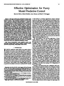
Fig. 1. Components of hydrological balance for an irrigation system relationship between water, soil and crop through the use of concepts like evapotranspiration and hydraulic balance; (2)the proposal of a predictive control design strategy applied to irrigation systems in order to optimize the use of water based on climatic factors while controlling the soil moisture level. The rest of this paper is structured as follows. Section 2 introduces the hydrological balance, the evapotranspiration and the soil moisture concepts. Then, in section 3 the formal definition of the process model is presented. Section 4 defines the controller design strategy. Section 5 describes the equipments and sensors used for process measurements. Section 6 presents the model parameter estimation based on direct measurements soil moisture and climatic conditions. Section 7 presents the results where the predictive model is evaluated against a traditional irrigation system based on the empirical definition of time periods, and against a basic soil moisture control system. Finally, section 8 concludes the paper. 2. PRELIMINARIES 2.1 Hydrological Balance The process dynamics of any agricultural irrigation system can be best described by using the hydrological balance model, depicted in Fig 1. This model establishes that a change in water storage during a time period in a specific location is the result of water inflows (irrigation, rainfall, capillary rise) minus the water outflows (evaporation, plant transpiration, water runoff and deep percolation), see Allen et al. [1998]. Using soil moisture θ in order to measure field water storage, then the hydrological balance dynamics can be defined as ˙ = ir(t) + rf (t) + cr(t) − etc (t) − dp(t) − ro(t), (1) θ(t) ˙ where soil moisture variations in the root zone θ(t) depends on effective irrigation ir(t), rainfall rf (t), capillary rise cr(t), crop evapotranspiration etc (t), deep percolation dp(t) and water outflow due run-off ro(t).
Crop evapotranspiration is a critical element in the hydrological balance for an irrigation system. Evapotranspiration represents the water lost caused by soil surface evaporation and crop transpiration. Evaporation and transpiration occur simultaneously and there is no easy way of distinguishing between the two processes. The evapotranspiration rate is normally expressed in millimeters (mm) per unit of time (usually days). The rate expresses the amount of water lost from the cropped surface in units of water depth. An evapotranspiration of 1mm/day is equivalent to a loss of 10, 000liters per hectare per day. Crop evapotranspiration etc depends on both, weather factors (soil radiation, temperature, humidity, wind velocity) and crop-soil characteristics (crop type, development stage, soil type, land fertility). Therefore, the water demand of any crop can be computed by multiplying the climatic factors of the evapotranspiration with a coefficient that depends on the crop specific characteristics, as denoted by etc (t) = Kc eto (t), (3) where eto (t) is the reference evapotranspiration that depends only on climatic parameters, and Kc is a constant that is known as the crop coefficient. To determine the crop coefficient Kc value, it is necessary, for to know the crop type, the total length of the growing season and the lengths of the various growth stages. This enables the transfer of standard values for Kc between locations and between climates. This has been a primary reason for the global acceptance and usefulness of the crop coefficient approach. The reference evapotranspiration eto is defined as the rate of evapotranspiration from a large area, covered by green grass, 8 to 15 cm tall, which grows actively, completely shades the ground and which is not short of water, further details can be found on Allen et al. [1998]. As stated by Soundar rajan et al. [2010], the eto estimation methods can be roughly classified as: temperature methods and radiation methods.
If a dry and plain land area for irrigation is considered, then rf (t) (assuming no rainfall), cr(t) (assuming no deep 4430
• The temperature methods assume that air temperature is directly proportional to the reference evapotranspiration; therefore in most of the cases the only measured variable is the temperature. Examples of these methods are: Blaney-Criddle, FAO BlaneyCriddle and Thornwaite. • The radiation methods consider that reference evapotranspiration depends mostly on solar radiation, although most of these methods also consider other variables (temperature included) for measurement.
19th IFAC World Congress Cape Town, South Africa. August 24-29, 2014
10 Blaney−Criddle FAO Blaney−Criddle Hargreaves Thornthwaite Penman−Monteith
9 8
ETo mm/day
7 6 5 4
Fig. 3. Irrigation system input/output definition
3 2 1 0 1
2
3
4
5
6
7
8
9
10
11
12
Month
Fig. 2. Monthly ETo for Chihuahua, M´exico based on 2012 climatological data Examples of these methods are: Hargreaves and FAO Penman-Monteith. According to Guevara [2006] the FAO Penman-Monteith is considered the most accepted method by the scientific community, since it is physically based and explicitly incorporates both physiological and aerodynamics parameters. Figure 2 shows the monthly reference evapotranspiration (eto ) for Chihuahua, M´exico, based on climatological data from year 2012, and calculated with different estimation methods. It can be denoted that for Chihuahua climatological conditions, a simpler FAO Blaney-Criddle estimation can be used instead of the accurate and more complex FAO Penman-Monteith, if solar radiation data is not available. Moreover, if air temperature is the only available variable then Blaney-Criddle may even provide a good approximation. 2.3 Soil Moisture Soil moisture refers to the amount of water in soil, which is described as the volumetric water content. Volumetric water content (θ) indicates the percentage of water volume for a specific volume: VW θ= , (4) VT where VW is the water content in volume units for a specific sample and VT is the total volume sample (soil + water + air). In any crop, the soil moisture needs to be maintained above permanent wilting point and stay below field capacity. Permanent wilting point is the soil moisture level at which plants cannot longer absorb water from the soil. Field capacity is the quantity of water stored in a soil volume after drainage of gravitational water. The available water capacity of soil is the water that is available to the crop, and it represents the range of soil moisture values that lie above permanent wilting point and below the field capacity. Field capacity and permanent wilting point are heavily influenced by soil textural classes, Rowell [1994], e.g. a silt loam type of soil (frequently used for agricultural purposes) has a typical value of 0.3 volumetric water content (V W C) for the field capacity, meanwhile the permanent wilting point typically has a value of 0.15.
In automated agriculture irrigation system, the most accurate irrigation schedules use regional etc forecasts in combination with soil moisture sensors to ensure that the soil moisture values stay at a level that is best for the crop health and yields. The evapotranspiration forecasts help the irrigator to create a weekly irrigation schedule, while soil moisture data takes into account microclimates and soil conditions and fine tune the weekly schedule on a daily basis. 3. PROCESS MODEL Based on the hydrological balance (2), the process dynamics for an irrigation system can be described by a block diagram with two inputs (effective irrigation and reference evapotranspiration) and one output (soil moisture), as shown in Fig. 3. Notice that reference evapotranspiration (eto ) is used instead of crop evapotranspiration (etc ), due eto depends only on external climatic parameters. By the other hand, etc is the result of eto that multiplies the crop coefficient (Kc ) according to (3), so it is assumed that Kc belongs to the internal process dynamics of the irrigation system. Also notice that deep percolation dp(t) is not present in the block, since it is assumed that water percolation in an irrigation system is clearly proportional to soil moisture, see Ooi et al. [2008], then (2) can be rewritten as ˙ = ir(t − τ ) − Kc eto (t − τ ) − c1 θ(t), θ(t) (5) where c1 is a constant value denoting the proportional relation between soil moisture and deep percolation, and τ represents the time-delay form the start of irrigation until the sensor detects a change in the soil moisture. Now, the process dynamics of any linear and continuoustime system, can be described by using the standard representation of a state-space model, x(t) ˙ = Ax(t) + Bu(t) (6) y(t) = Cx(t), where x(t) is a vector of a state variables (state of the process), u(t) is the control signal or process input, y(t) is the process output; A, B, C are constant matrices that describes the dynamics of the process. Therefore (5) can be reformulated by using a first-order state-space representation as [ ] ir(t − τ ) ˙ θ(t) = A [θ(t)] + B eto (t − τ ) (7) y(t) = C [θ(t)] , soil moisture (θ) is the state variable; effective irrigation ir and reference evapotranspiration eto are the process inputs. Notice that an input time delay has been included (τ ) in order to model the period of time since the irrigation starts until the sensor detects a change in the soil moisture.
4431
19th IFAC World Congress Cape Town, South Africa. August 24-29, 2014
Fig. 5. Equipment and sensors used for measurements 5. MEASURING EQUIPMENT Fig. 4. Model predictive control loop Constant Kc and c1 , have been absorbed by matrices B and A respectively. By using generic constant for A, B and C matrices, then the complete state-space representation is given by [ ] ˙θ(t) = [−c1 ] [θ(t)] + [c2 − c3 ] ir(t − τ ) eto (t − τ ) (8) y(t) = [1] [θ(t)] , where c1 , c2 and c3 are constants that defines the dynamics of the process and can be obtained from direct measurements of the evapotranspiration, the soil moisture and the effective irrigation.
Soil measurements were conducted by using a Decagon 1 EC-5 volumetric water content sensor. The sensor was located in a depth of 20cm in order to measured the soil moisture at the grass root level. The grass grows over a silt loam type of soil whose field capacity and permanent wilting point are 0.30 V W C and 0.15 V W C respectively, therefore 0.18 V W C is considered as an adequate soil moisture set-point in order to avoid water stress. A Decagon VP-3 air temperature sensor was used to calculate hourly eto based on Blaney-Criddle method and is located in-field near to the soil moisture sensor. Both sensors are connected into a Decagon EM50R Wireless Data Logger, then data is transmitted to a remote data station (Decagon ECH20) that is connected via serial port to a personal computer. Soil moisture and air temperature data are stored and plotted in the computer using the Decagon DataTrac software, as shown in Fig. 5.
4. CONTROLLER DESIGN
6. MODEL SIMULATION
A model predictive control (MPC) can be used in order to minimize the control signal (effective irrigation) while keeping soil moisture under specific thresholds (avoiding water stress) and by considering external disturbances (reference evapotranspiration) predict the process dynamics. Figure 8 shows a feedback loop where the control objective is to keep within certain thresholds the soil water content in order to have a healthy and productive crop. Thus the process variable y(t) is the soil moisture, r(t) is the reference value (soil moisture set-point), and the error value e(t) is obtained as a result of the difference between the process value and the reference value.
Process dynamics model defined by (8) has been simulated using Matlab 2 . In order to validate the theoretical model the simulation of the process dynamics has been compared with data obtained directly from soil moisture, effective irrigation and evapotranspiration measurements. The process dynamics coefficients c1 , c2 and c3 from (8) were estimated from direct measurements using the Matlab system identification toolbox.
The climatic factors affecting the irrigation systems are modelled as an external disturbance, and the reference evapotranspiration eto represents the disturbance signal affecting the process. By knowing the disturbance model, then the system may predict the disturbance effects and react before these effects affect the process output. The controller knows the process dynamics due the internal model. Within the controller, an numerical optimization algorithm is executed based on the current error and the disturbance measurements, this information is applied to the internal model and an optimal solution is found over a finite horizon TF H , which minimizes a cost function based on the error e(t) and the control signal u(t), ∫
f (e(t), u(t))dt. t=0
The measurement and simulation conditions considered were: one hectare of grass (eto = etc ) irrigated once every two days approximately, with a daily average evapotranspiration of 7.76 mm/day (typical value for the month of May in Chihuahua, Mexico), each irrigation event has a duration of 0.5 hours in order to keep the soil moisture above of 18%, and finally a process input time-delay of 0.1 hours is considered. Reference evapotranspiration has a periodical behavior i.e. eto is low at night and is high during the day, reaching the maximum value at noon and the minimum value at midnight and early morning. Effective irrigation takes place 1
TF H
minimize J =
For validation purposes hourly sampling periods are considered and a total of 48 hours (2 days) were simulated and compared against direct measurements. Figure 6 shows the process output comparison (soil moisture θ) during the validation period, in general the model output provides an adequate approximation according to the measured data.
(9)
Decagon Devices, http://www.decagon.com Matlab is a product developed http://www.mathworks.com 2
4432
by
Mathworks
19th IFAC World Congress Cape Town, South Africa. August 24-29, 2014
Fig. 6. Model dynamics simulation data against measured data Fig. 7. Accumulated error evaluation the first day in the morning and it is modelled as a short pulse signal, since real irrigation last only few minutes but provides great amount of water. As for the soil moisture (process output), it increases suddenly after an irrigation event, then it decreases slowly due evapotranspiration. Soil moisture slope, represent the water depletion, and it is higher during the day (high eto ) and lower during the night (low eto ). Based on the validation results, it can be derived that an irrigation system can be described by a process block with two inputs (effective irrigation and reference evapotranspiration) and one output (soil moisture), where reference evapotranspiration depends on climatic external factors and effective irrigation can be considered as the control signal, meanwhile process output (soil moisture) can be measured by using adequate sensors.
7. MODEL EVALUATION In order to identify the potential impact of the use of a MPC in the process dynamics, simulations were conducted to evaluate three different types of irrigation methods: (1) Time-based irrigation, where an open-loop periodical irrigation is implemented, the irrigation period and the duration of each irrigation event is determined empirically. (2) Soil moisture control-based irrigation, a simple on-off closed loop control system is implemented in order to maintain soil moisture within pre-defined thresholds. (3) Model predictive control-based irrigation, this schema includes a closed loop control to maintain soil moisture within predefined thresholds and a predictive model based on the process dynamics and the disturbance measurements. The three irrigation methods are compared in terms of accumulated error Jacum and control effort Jcontrol . The accumulated error indicates how good the system is to maintain the soil moisture levels close to the reference value. The control effort indicates how efficient the system is, in order to minimize the water consumption. In both cases, the lower the value the better the performance. These parameters are defined as
T∫sim
|e(t)|,
Jacum =
0 T∫sim
(10)
|u(t)|,
Jcontrol = 0
where Tsim is the simulation time, e(t) is the difference between the soil moisture reference value and the process output (current soil moisture), and u(t) is the control signal (effective irrigation). In Fig. 7 the accumulated error of the three irrigation methods is shown, it can be observed that the MPC controller has a better performance since the accumulated error is the lowest. The on-off controller has the worst behavior, since this simple schema does not account for the input process time delay. By the other hand, the MPC controller includes in its internal model the input timedelay, therefore is more robust to timing variations. In Fig. 8 the control effort of the three irrigation methods is compared. These is a critical parameter since it represents the system water consumption. It can be observed that the highest water consumption is provided by the openloop system, since no feedback information is provided to the controller, and then the control signal is sent periodically even when the process does not require it. The on-off control improves water consumption by keeping the soil moisture within predefined levels. However the lowest water consumption is provided by the MPC controller, since an internal optimization algorithm allows to reduce the control effort. In general the MPC controller potentially offers the best performance considering the reference error and the control effort parameters. The implementation MPC controller requires an intensive computational load, however the capability of new embedded devices makes feasible the implementation of complex algorithm such as the required in an MPC controller. Also the relatively slow process dynamics for an irrigation system makes feasible the implementation of this predictive control strategy. 8. CONCLUSIONS This paper proposes the use of a predictive control strategy for a closed-loop irrigation control model. Considering
4433
19th IFAC World Congress Cape Town, South Africa. August 24-29, 2014
Fig. 8. Control effort evaluation that the process dynamics of an irrigation system can be described with the hydrological balance model, where evapotranspiration and soil moisture represents the model main variables, then a model predictive control (MPC) can be used in order to minimize the control signal (effective irrigation) while keeping soil moisture under specific thresholds (avoiding water stress) and considering external disturbances (reference evapotranspiration) to predict the process dynamics. The proposed model has been simulated and compared against direct measurements from an irrigation system for validation purposes. Then the proposed control strategy has been evaluated against more conventional irrigation methods. Simulation results indicate that the use of a model predictive control in an irrigation system, achieves a higher control efficiency and significantly reduce the control effort (water consumption). Future work will focus on the implementation of the proposed controller in an embedded device in order to perform experimental evaluations with different control algorithms and validate the feasibility of a predictive control strategy in an irrigation system. ACKNOWLEDGEMENTS Special thanks to the “Fondo Mixto de Fomento a la Investigaci´ on Cient´ıfica y Tecnol´ogica CONACyT - Gobierno del Estado de Chihuahua, M´exico” for funding this project. REFERENCES Allen R.G., Pereira L.S., Raes D., and Smith M., Crop evapotranspiration: Guidelines for computing crop water requirements. FAO Irrigation and Drainage Paper 56. FAO - Food and Agriculture Organization of the United Nations. Rome, Italy, 1998. Constantinos M.A., Sotiris E.N. and Georgios C.T., A Smart System for Garden Watering using Wireless Sensor Networks. ACM MOBIWAC 2011, Miami, USA, 2011. Guevara-Diaz J.M., The Use of the 1998 PenmanMonteith FAO Formula in order to Determine Referential Evapotranspiratio. Terra, Vol XXII, No. 31, pp 31-72, 2006. Kijne J.W., Molden D. and Barker R., Water productivity in agriculture: limits and opportunities of improvement. Comprehensive assessment of water management
in agriculture series, No. 1 Wallingford, UK, CABI Publishing, 2003. Kim Y., Evans R.G. and Iversen W.M. Remote Sensing and Control of an Irrigation System Using a Distributed Wireless Sensor Network. IEEE TRansactions on Instrumentation and Measurement, vol 57, no. 7, July 2008. Kim Y., Evans R.G. and Iversen M.V., Evaluation of Closed-Loop Site Specific Irrigation with Wireless Sensor Network. Joournal of Irrigation and Drainage Engineering,ASCE, January-February 2009. Kulkarni S., Innovative Technologies for Water Saving in Irrigated Agriculture. International Journal of Water Resources and Arid Environments 1(3): 226-231, 2011 ISSN 2079-7079 Li Z., Wang N., Hong T.S., Franzen A. and Li J.N., Closedloop drip irrigation control using a hybrid wireless sensor and actuator network. Science China / Information Sciences. Vol. 54 No. 3: 577-588, March 2011. Maciejowski J. Predictive Control with Constraints. Prentice-Hall, 1st Edition, 2000. Ooi S.K., Mareels I., Cooley N., Dunn G. and Thoms G, A Systems Engineering Approach to Viticulture On-Farm Irrigation. Proceedings of the 17th World Congress. The International Federation of Automatic Control, Seoul, Korea, July 2008. Overloop P.J., Model predictive control on open water systems. Delft University of Technology, IOS Press, ISBN: 1-58603-638-6, 2006 Pfitscher L.L., Bernardon D.P., Kopp L.M., Heckler M., Behrens J., Montani P.B. and Thome B., Automatic control of irrigation systems aiming at high energy efficiency in rice crops. Devices, Circuits and Systems (ICCDCS), 8th International Caribbean Conference, pp.1,4, 14-17 March 2012 Puig V., Ocampo-Martinez C:, Romera J., Quevedo J., Rodriguez P., de Campos S. and Negenborn R.R., Model predictive control of combined irrigation and water supply systems: Application to the Guadiana river. IEEE International Conference on Networking, Sensing, and Control (ICNSC 2012), Beijing, China, April 2012. Renault D. and Wallender W.W., Nutritional water productivity and diets: from crop per drop to nutrition per drop. Agriculture water management, 45:275-296, 2000. Rowell, D. L., Soil Science Methods and Applications. John Wiley and Son Inc. 1994. Soundar rajan D., Vijayalakshmi M.M., Nethaji Mariappan V.E., Assessing a Suitable Method in Estimating Evapotranspiration for Crop Water Requirement. Recent Advances in Space Technology Services and Climate Change (RSTSCC), 2010 Water Report, The United Nations World Water Development Repor. UNESCO publishing, 2003. http://www.unseco.org/water/wwap. Yuan Y.W., Zhang X.C. and Zhao H.P., Study on precision irrigation technology of large scale irrigator. ComputerAided Design and Computer Graphics, CADGraphics 09 11th IEEE International Conference, 2009. Zhao Y., Bai C. and Zhao B., An Automatic Control System of Precision Irrigation for City Greenbelt. IEEE Conference on Industrial Electronics and Applications, 2007.
4434