An example of an open-loop system is gas flow through an aircraft engine. On the other hand, if the ... cardio-vascular circulatory system. Boundary conditions ...
Model Predictive Optimal Control of a Time-Delay Distributed-Parameter System Nhan Nguyen∗ NASA Ames Research Center, Moffett Field, CA 94035 This paper presents an optimal control method for a class of distributed-parameter systems governed by first order, quasilinear hyperbolic partial differential equations that arise in many physical systems. Such systems are characterized by time delays since information is transported from one state to another by wave propagation. A general closed-loop hyperbolic transport model is controlled by a boundary control embedded in a periodic boundary condition. The boundary control is subject to a nonlinear differential equation constraint that models actuator dynamics of the system. The hyperbolic equation is thus coupled with the ordinary differential equation via the boundary condition. Optimality of this coupled system is investigated using variational principles to seek an adjoint formulation of the optimal control problem. The results are then applied to implement a model predictive control design for a wind tunnel to eliminate a transport delay effect that causes a poor Mach number regulation.
I. Introduction The terminology of distributed-parameter system is used to describe physical systems whose state variables are functions of both space and time that are usually modeled by partial differential equations (PDEs). Optimal control of distributed-parameter systems has been studied extensively in mathematical literature, but applications of this type of control are limited in practical control engineering. Hyperbolic PDEs are used to model transport systems whose information is carried from one point to another within those systems as a function of space and time.1 Examples of transport systems are numerous in many physical applications such as fluid flow in gas distribution pipelines,2 air traffic systems,3 highway traffic systems,4 to name a few. These equations describe wave propagation that exists in transport systems to propagate information from one point to another within the continuum. A characteristic of a hyperbolic system is time delay which describes a finite time that information is transported from one location to another. Consider the simplest hyperbolic equation ∂y ∂y +a =0 ∂t ∂x The solution of this equation is
(1)
� x� (2) y =f t− a Equation (2) describes the solution of a wave of a transport process that propagates at a wave speed a and the term x/a is a variable transport time delay. As with any PDEs, boundary conditions are used to specify configurations of these transport systems. If the information is carried in one direction without returning to its starting position, then we say that the system is openloop. An example of an open-loop system is gas flow through an aircraft engine. On the other hand, if the information returns to its starting position, then the system is said to be closed-loop. An example of a closed-loop system is the cardio-vascular circulatory system. Boundary conditions associated with closed-loop systems are usually periodic in nature. The flow of information is usually supplied at the system boundary by a forced process that provides a motive force to move the information along the way by wave propagation. For example, a common device for accomplishing this objective in fluid transport systems is a pump which supplies a positive pressure head to displace the fluid volume ∗ Computer
Scientist, Intelligent Systems Division, Mail Stop 269-1 1 of 16 American Institute of Aeronautics and Astronautics
in the flow direction. Such a process whereby the control is applied at the boundary of the continuum is called a boundary control process. In real systems, boundary control processes are often governed by other auxiliary dynamical processes. For example, a positive-displacement pump may be driven by an electrical motor that imposes a constraint on the pump speed according to the motor torque dynamics. The pump speed in this case is a boundary control variable. In this study, we present an optimal control method for a class of closed-loop hyperbolic distributed-parameter systems whose boundary control process is constrained by a dynamical system governed by a nonlinear ordinary differential equation (ODE) via a periodic boundary condition. The optimal control problem is formulated by an adjoint method to seek necessary conditions for optimality via calculus of variations. The theory is then used to develop a model predictive linear-quadratic regulator optimal control that results in a modified Riccati equation. The model predictive control computes control inputs based on model information at the current time that need to be apply ahead of error signals in order to minimize system disturbances due to time delays. Thus, it is effectively a feedforward control. We apply this theory to solve a flow control problem in a wind tunnel.
II. Problem Formulation Transport phenomena are governed by the conservation laws equations which dictate the conservation of some quantities such as traffic density, mass flux, and enthalpy. These equations are generally hyperbolic in nature. For a 1-D system, these equations are expressed in a conservation form as5 ∂y ∂F (y, x) + + Q (y, x) = 0 ∂t ∂x
∀x ∈ [0, L] , t ∈ [0, tf ]
(3)
where y (x, t) : [0, L] × [0, tf ] → Rn in class C 1 is a vector of conserved quantities, F (y, x) is a flux function, and Q (y, x) is a non-homogeneous source term. By explicit differentiation, Eq. (3) can be rewritten in as ∂y ∂y + A (y, x) + B (y, x) = 0 ∂t ∂x
∀x ∈ [0, L] , t ∈ [0, tf ]
(4)
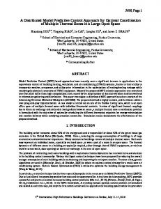
where A (y, x) : Rn × [0, L] → Rn × Rn is a characteristic matrix such that A (y, x) = Fy (y, x) and B (y, x) : Rn × [0, L] → Rn is a non-homogeneous source term such that B (y, x) = Q (y, x) + Fx (y, x). Equation (4) is a system of first order, quasilinear hyperbolic equations due to the fact that the matrix A has n real, distinct eigenvalues such that λ1 (A) < λ2 (A) < . . . < λm (A) < λm+1 (A) < λm+2 < . . . < λn (A) for all y (x, t) ∈ Rn , x ∈ [0, L], and t ∈ [0, tf ], where m < n are number of negative eigenvalues of A. The eigenvalues are the wave speeds of the transport system and the direction of the wave propagation is called a characteristic direction. If m > 0, the information in the continuum is carried in both the upstream and downstream directions by negative wave speeds λi , i = 1, 2, . . . , m and positive wave speeds λi , i = m + 1, m + 2, . . . , n; respectively. If the solution domain is 0 ≤ x ≤ L, then for the information to be transported in the upstream direction by the negative wave speeds, information must exist at the boundary x = L. Similarly, information must also exist at the boundary x = 0 in order for the information to be carried downstream by the positive wave speeds. Therefore, the number of upstream and downstream boundary conditions must match the number of negative and positive eigenvalues. This is known as the boundary condition compatibility. In a closed-loop transport system, information is carried from one point to another and then returned back to the starting position as illustrated in Fig. 1. To enable this information flow, a periodic boundary control process is embedded within the system. For a closed-loop system, the boundary conditions at x = 0 are affected by the boundary conditions at x = L since the information must be returned to its starting position. Thus, in general for a closed-loop system, we specify the following general nonlinear periodic boundary condition for Eq. (4) y (0, t) = g (y (L, t) , u (t))
∀t ∈ [0, tf ]
(5)
where u (t) : [0, tf ] → Rm in class C 1 is a boundary control vector, and g (y (L, t) , u) : Rn × Rm → Rn is a nonlinear forcing function that relates the transport state vectors at x = 0 and x = L and the boundary control vector u. 2 of 16 American Institute of Aeronautics and Astronautics
Fig. 1 - Closed-Loop Transport Model To ensure the boundary condition compatibility for all signs of eigenvalues, the Fréchet derivative or the Jacobian of g with respect to y (L, t) is required to have a full rank or � � dim gy(L,t) = n (6) In many real systems, boundary control processes are actually controlled by other auxiliary processes. These auxiliary processes may be dynamical so that their dynamics can be described by a nonlinear ODE u˙ = f (y (0, t) , y (L, t) , u, v)
(7)
where v (t) : [0, tf ] → Rl is an auxiliary control vector that belongs to a convex subset of admissible auxiliary control Vad ⊆ Rl , and f (y (0, t) , y (L, t) , u, v) : Rn × Rn × Rm × Rl → Rm is a nonlinear function. Thus the auxiliary control vector v actually influences the boundary control vector u, which in turn controls the behavior of the closed-loop transport system described by Eq. (4) and the periodic boundary condition (5).
III. Optimal Control Theory Optimal control and optimization theories of hyperbolic systems has been studied extensively in mathematical literature. Within the theoretical framework of systems governed by PDEs, control of such systems can exist as distributed control, boundary control, interior pointwise control, or others. Hou and Yan studied the long time behavior of solutions for an optimal distributed control problem for the Navier-Stokes equations.6 Nguyen et al investigated a flow control problem with interior pointwise control.7 Optimal control problems of transport systems with boundary control have been examined for many different types of constraints imposed on either state or control variables. Raymond and Zidani investigated necessary optimality conditions in the form of a Pontryagin’s minimum principle for semilinear parabolic equations with pointwise state constraints and unbounded control.8 Casas et al established second order sufficient conditions for local optimality of elliptic equations with pointwise constraints on the boundary control and equality and set-constraints on state variables.9 Kazemi obtained adjoint equations for a degenerate hyperbolic equation.10 Adjoint method is well-known in optimal control and optimization theories as it provides an indirect method for solving optimization problems. For a transport system governed by hyperbolic equations, two types of adjoint formulation are used: discrete adjoint and continuous adjoint. Any hyperbolic equation can generally be discretized into a system of ODEs by means of numerical discretization techniques such as finite-difference or finite-element methods. If the adjoint method is formulated with the discretized hyperbolic equations, then this is known as discrete adjoint method. On the other hand, continuous adjoint method is normally applied directly to the original hyperbolic equations. This method has been used in aerodynamic design optimization studies involving the Euler and NavierStokes equations.11 Nadarajah et al compared the discrete and continuous adjoint methods in aerodynamic design optimization and suggested that the continuous adjoint method affords a certain advantage over the discrete adjoint method for Navier-Stokes flow problems.12 In the present study, we apply this method to the present hyperbolic system with nonlinear differential equation constraints on a periodic boundary condition. To formulate the continuous adjoint method for this system, we seek a solution of the hyperbolic system above that minimizes the following multi-objective cost functional Z T Z tf Z L � (8) L1 (y) dxdt + L2 y0 , yL , u, v dt min J (y, u, v) = 0
0
0
3 of 16
American Institute of Aeronautics and Astronautics
where L1 is an objective function defined over the continuum of the transport system, L2 is an objective function defined on the system boundary, and the superscripts 0 and L are short hand notations denoting the associated vector quantity evaluated at x = 0 and x = L, respectively. The following assumptions are required: (A1): Eq. (4) admits smooth solutions for shock-free conditions. (A2): v ∈ L2 , the space of real value functions in Rl for which the norm kvk is square-integrable. (A3): The Fréchet derivatives of L1 , L2 , B, g, and f with respect to y, y0 , yL , u, and v exist and are bounded so as to satisfy the Lipschitz condition. We note that Eq. (4) also has discontinuous solutions known as entropy solutions14 which will not be treated here. The transport system above is posed as a boundary control problem of hyperbolic equations with nonlinear differential equation constraints. Lemma 1: Let D be a nonlinear differential operator and D∗ be its adjoint differential operator such that for some z (x, t) ∈ Rn and λ (x, t) ∈ Rn ∂z Dz = A ∂x � ∂ A> λ D∗ λ = ∂x where the superscript > is the transpose operator, then the following inner product operation in L2 is equivalent D D �L E �0 E hDz, λi(x,t) = − hz, D∗ λi(x,t) + zL , A> λ − z0 , A> λ (9) t
t
Proof: The inner product hDz, λi(x,t) in L2 is
Z
hDz, λi(x,t) = Integrating by parts yields Z Z tf Z L λ> Dzdxdt = − 0
0
0
tf
Z
tf
Z
0
L
λ> Dzdxdt
0
L
z> D∗ λdxdt +
Z
tf
0
0
h
We define the following inner products D
zL , A> λ
�L E
t
Z D �0 E − z0 , A> λ = t
tf
0
h
zL
�>
zL
�>
AL
AL
�>
�>
λL − z0
λL − z0
�>
�>
A0
�>
A0
�>
i λ0 dt
i λ0 dt
Equation (9) is thus obtained. Definition 1: Let F : X → Y be a functional with X, Y in Banach spaces and α ∈ X. If there exists a continuous linear operator ∇F (α) : X → Y for any variation δ ∈ X such that
F (α + εδ) − F (α)
=0 ∇F (α) δ − lim
ε→0 ε
then ∇F (α) is called a Gâteaux derivative of F at α.16 Definition 2: The following Hamiltonians are defined
H1 (y, x, λ) = L1 − λ> B � H2 y0 , yL , u, v, µ = L2 + µ> f
(10) (11)
We are now ready to state the necessary conditions for optimality. ¯, v ¯ ) is an optimal solution of Eq. (8), then there exist adjoint Theorem: If (A1)-(A3) are fulfilled and if (¯ y, u variables λ (x, t) : [0, L] × [0, tf ] → Rn and µ : [0, tf ] → Rk that satisfy the following dual adjoint system � > λt + A> λ x + H1,y =0 �L �0 > > > > > > (12) A λ = H2,yL + gyL A λ + gyL H2,y0 λ (x, tf ) = 0 4 of 16
American Institute of Aeronautics and Astronautics
) �0 > > µ˙ = −H2,u − gu> A> λ − gu> H2,y 0 µ (tf ) = 0
(13)
with a terminal time transversality condition Z
0
L
L1 |t=tf dx + L2 |t=tf = 0
(14)
such that the optimal control is one that satisfies the following Pontryagin’s minimum principle � ¯ = arg min H2 y¯0 , y¯L , u ¯ , v, µ v
(15)
v∈Vad
¯ ) in variations for a variation q in v ¯ , then the variation in the cost Proof: Let α = (z, p) be solutions to β = (¯ y, u functional from Eq. (8) is computed as ¯ + q) − J (β, v ¯) > 0 ∆J (q) = ∇J (β) + J (β, v
where the Gâteaux derivative of J at β is evaluated as
> �
> � 0 ∇J (β) = H1,y , z (x,t) − hλ, zt i(x,t) − hλ, Dzi(x,t) + H2,y 0, z t
Z D E
> � > L ˙ t + δt + H2,u , p t − hµ, pi + H2,yL , z t
0
L
L1 |t=tf dx + L2 |t=tf
!
From the boundary condition (5), we have the following variations z0 = gy>L zL + gu> u From Lemma 1 and the variations in the boundary condition (5) plus vanishing variations in initial conditions for Eqs. (4) and (7), this becomes D
� �L E �0 > > > > > > ∇J (β) = λt + D∗ λ + H1,y , z (x,t) −hz (x, tf ) , λ (x, tf )ix + gy>L H2,y ,z + H2,y 0 + gy L A λ L − A λ t ! Z L D E � 0 > > ˙ > , p − µ> (tf ) p (tf ) + δt L1 |t=tf dx + L2 |t=tf + gu> A> λ + gu> H2,y 0 + H2,u + µ t
0
Setting ∇J (β) = 0 for arbitrary variation α results in Eqs. (12)-(14). Then the variation in the cost functional becomes Z tf Z tf � � � � � � ¯0, y ¯L, u ¯ + q, µ − µ> u ¯0, y ¯L, u ¯ , µ − µ> u ∆J (q) = ¯, v ¯˙ dt − H2 y ¯, v ¯˙ dt > 0 H2 y 0
0
This leads to the Pontryagin’s minimum principle
� � ¯0, y ¯L, u ¯ + q, µ > H2 y ¯0 , y ¯L, u ¯, µ H2 y ¯, v ¯, v
for all values of the variation q. Equation (15) is the equivalent Weierstrass condition for strong variations. For weak variations when v is unconstrained and L1 and L2 are convex, the Pontryagin’s principle leads to the Legendre-Clebsch condition15 ) � ¯0, y ¯, v ¯, µ = 0 H2,v y ¯L , u � (16) ¯L, u ¯, v ¯, µ > 0 H2,vv y ¯0 , y
5 of 16 American Institute of Aeronautics and Astronautics
IV. Linear-Quadratic Optimal Control for Scalar Hyperbolic Systems Linear advection hyperbolic equations are used to model some transport processes that involve small-amplitude wave propagation in only one direction such as pressure wave propagation in a fluid continuum. Our objective is to develop a linear-quadratic regulator (LQR) for the following linear advection equation ∂y 1 ∂y + + β (x, t) y + w (x, t) = 0 α (x) ∂t ∂x
(17)
where y (x, t) ∈ R is a transport state variable, α (x) > 0 is the wave speed, β (x, t) is a dissipative term, and w (x, t) is a disturbance. Equation (17) is subject to a zero initial condition and a periodic boundary condition for a closed-loop system y (0, t) = Gu (t) + Hy (L, t)
(18)
where u (t) ∈ Rm is a boundary control vector, G : R → R × Rm is a constant-valued matrix, and H is a constant. The following linear dynamics is imposed on the boundary control vector u with a zero initial condition u˙ = Cu + Dv + Ey (0, t) + Fy (L, t)
(19)
where C : R → Rm × Rm is a constant-valued state transition matrix, D : R → Rm × Rl is a constant-valued control transition matrix, and E and F are constants. We want to minimize the following linear-quadratic cost functional with respect to v for a fixed final time tf � Z tf � 1 2 1 > 1 > P y (0, t) + u Qu + v Rv dt (20) min J = 2 2 2 0 where P ≥ 0, Q ≥ 0, and R > 0 are weighting factors. The dual adjoint systems from (12) and (13) for the optimal control problem are given as ∂ ∂λ + (αλ) − βαλ = 0 ∂t ∂x
(21)
� α (L) λ (L, t) = Hα (0) λ (0, t) + HP y (0, t) + F> + HE> µ � µ˙ = −Qu − C> + G> E> µ − G> α (0) λ (0, t) − G> P y (0, t)
(23)
Rv + D> µ = 0
(24)
(22)
with the transversality conditions λ (x, tf ) = 0 and µ (tf ) = 0 along with the stationary condition obtained from Eq. (16)
Equations (17)-(19) and (21)-(23) form a two-point boundary value PDE-ODE problem. Even though the PDEs are linear and scalar, the two-point boundary conditions (18) and (22) pose a challenge in obtaining a general feedback control solution. To see this, we solve Eq. (17) using the characteristic method which yields the following solution ( 0 t < td (x) y (x, t) = (25) a (x, t) [f (t − td (x)) − q (x, t)] t ≥ td (x) where td (x) is a variable transport time delay, a (x, t) is a wave decay factor, and q (x, t) is a forcing function due to the disturbance w (x, t) Z x dσ td (x) = 0 α (σ) � Z x � a (x, t) = exp − β (σ, t − td (x) + td (σ)) dσ 0
q (x, t) =
Z
0
x
w (σ, t − td (x) + td (σ)) dσ a (σ, t − td (x) + td (σ)) 6 of 16
American Institute of Aeronautics and Astronautics
The function f (t − td (x)) represents the wave propagation and must be determined from the boundary condition (18) as f (t) = Gu (t) + Ha (L, t) [f (t − td (L)) − q (L, t)] (26) Let T = td (L) be a transport delay period, then Eq. (25) has a series solution " k−1 # " k # n n X Y X Y f (t) = Gu (t) + Ha (L, t − mT ) Gu (t − kT ) − Ha (L, t − mT ) q (L, t − kT ) k=1
m=0
k=0
Similarly, the solution of Eq. (20) is given as ( α (x) λ (x, t) =
(27)
m=0
0 τ < τd (x) − τd (x)) τ ≥ τd (x)
(28)
a(L,t) a(x,t) g (τ
where τ = tf − t, τd (x) = T − td (x), and g (τ ) = HP y (0, t) + HP
" k−1 n Y X
k=1
m=0
#
� Ha (L, t + mT ) y (0, t + kT ) + F> + HE> µ (t) >
+ F + HE
>
" k−1 n Y �X k=1
#
Ha (L, t + mT ) µ (t + kT ) (29)
m=0
Equations (27) and (29) illustrate the nature of a closed-loop transport system whereby the solutions are expressed as time-shifted series of the transport delay period. The resulting ODEs (19) and (22) thus will contain the time-shifted series. Therefore, in general a feedback control is difficult to obtain. Nonetheless, there are two simplified solutions in the limit that we need to consider. The first case is associated with a short time horizon when tf < T , for which λ (0, t) = 0 from Eq. (29) since the system must be causal. Then, we get from Eqs. (27) and (29) y (0, t) = Gu (t) − Ha (L, t) q (L, t)
(30)
y (L, t) = −a (L, t) q (L, t)
(31)
The second case is associated with an infinite time horizon when tf → ∞, for which f (t − T ) ' f (t) and g (τ − T ) ' g (τ ). The infinite time horizon case is possible if the time scale of the linear advection equation is much greater than the time scale of the ODE. Equivalently, this time scale separation results in |α (x)| � ρ (C), where ρ is the spectral radius of the matrix C. Utilizing the series identity ∞
X 1 = H k ak (L) 1 − Ha (L)
(32)
k=0
we obtain y (0, t) =
Gu (t) − Ha (L, t) q (L, t) 1 − Ha (L, t)
a (L, t) [Gu (t) − Ha (L, t) q (L, t)] − a (L, t) q (L, t) 1 − Ha (L, t) � � � a (L, t) HP y (0, t) + F> + HE> µ (t) α (0) λ (0, t) = 1 − Ha (L, t)
y (L, t) =
(33) (34) (35)
In essence, the solution for any tf may be assumed to be bounded between these two cases. we introduce a factor γ that represents the effect of the time horizon such that 0 ≤ γ ≤ 1, with γ = 0 corresponding to the first case and γ = 1 corresponding to the second case. Then, we are now able to obtain a feedback control v in terms of the boundary control u and the transport states at the boundaries y (0, t) and y (L, t) v (t) = −R−1 D> Wu − R−1 D> Va (L, t) q (L, t) 7 of 16 American Institute of Aeronautics and Astronautics
(36)
where W and V are solutions of the following matrix Riccati equations using a backward sweep method by letting µ = W∆u + Va (L, t) q (L, t)
with
−1 > WCe + C> D W + Qe = 0 e W − WDR
(37)
Ce > V − WDR−1 D> V − WS − U = 0
(38)
Ce = C + EG + γ (F + EH) Ga (L, t) [1 − γHa (L, t)]−1 Qe = Q + G> P G [1 − γHa (L, t)]
−2
S = (F + EH) [1 − γHa (L, t)]−1 −2
U = G> P H [1 − γHa (L, t)]
We see that the optimal control solution of a linear advection equation has a form of a Riccati solution. The Riccati equation contains modified matrices that incorporate the dynamics of the linear advection equation. The control is a state feedback and a disturbance feedforward where the forcing function q (L, t) is the disturbance that is delayed by the time delay T . Thus, the control would not be responsive during this time delay. We note that the control can also be written in an output feedback form by noting that a (L, t) q (L, t) = γa (L, t) y (0, t) − y (L, t)
(39)
v (t) = −R−1 D> Wu − R−1 D> Vγa (L, t) y (0, t) + R−1 D> Vy (L, t)
(40)
so that
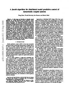
V. Flow Control Application We now apply the general theory to a flow control problem to regulate the test section Mach number in a closedcircuit wind tunnel. An example is the NASA Ames 11-Foot Transonic Wind Tunnel as shown in Fig. 2.
Fig. 2 - Closed-Circuit Wind Tunnel The fluid transport process in a closed-circuit wind tunnel is a good example of a closed-loop transport process whereby the fluid flow is recirculated through a compressor providing the boundary control action. The compressor is controlled by two auxiliary dynamical processes: a drive motor dynamics, and an inlet guide vane (IGV) angle dynamics. By controlling the drive motor speed and the IGV angle, the flow in the test section can be set as desired. iT h The full nonlinear model of this system is described by Eq. (4) with y (x, t) = m and ˙ p0 T 0
A=
u ρ0 c2 ρA (k−1)T ρA
pA p0 h u 1 − (k−1)T T0 (k−1)2 T u − kp0
i
h u 1
mu ˙ 2T0 ρ0 c2 u T0 + (k−1)T T0
, B = i
muξ ˙ h 2
kp0 u3 f 1 − (k−1)T 2c2 T0 (k−1)2 T u3 ξ − 2c2
i
where m ˙ is the mass flow, p is the pressure, T is the temperature , ρ is the density, u is the flow speed, c is the speed of sound, ξ is a loss factor, A is the cross sectional area, and the subscript 0 denotes the stagnation condition. 8 of 16 American Institute of Aeronautics and Astronautics
The compressor provides a boundary control action at x = 0 and x = L that results in a total pressure rise that recirculates the flow. Using an empirical model, we obtain the forcing function g in the periodic boundary condition (5) for the wind tunnel model as
g (y (L, t) , u) =
m ˙ (L, t) ! 4 2 P P p0 (L, t) 1 + cij θj ωci b1 − b2 i=2 j=0
n T0 (L, t) 1 +
h
b3 ωc m ˙c
p0 (0,t) p0 (L,t)
3 2 j i dij θ ωc i=1 ioj=0 −1 m˙ c
(41)
where ω is the compressor speed, θ is the IGV angle, and bi , cij , dij are empirical coefficients derived from experimental compressor performance measurements. The drive motors employ a drive motor speed control system that utilizes a variable resistance device known as rheostat to control the motor speed. By varying a rotor resistance Rr in the rheostat, the motor torque changes. The difference between the motor torque and the aerodynamic torque causes the motors to accelerate or decelerate according to the following equation Jm ω˙ =
Km Rr ωs (ωs − ω) 2
2
[Rs (ωs − ω) + Rr ωs ] + L2s ωs2 (ωs − ω)
− Ka [p0 (0, t) − p0 (L, t)]
(42)
where Jm is the motor inertia, Rs is the stator resistance, Ls is the stator inductance, ωs is the synchronous speed, Km is the motor torque constant, and Ka is the aerodynamic torque. The inlet guide vanes are adjustable with movable trailing edge flaps and are driven by DC field motors that are controlled by a field voltage Va according to the following equation � � 2 2 ni ρ (L, t) u2 (L, t) bf c2f CH KT KE ˙ ni ρ (L, t) u (L, t) bf cf CH,θ KT Va b+ θ+ θ = − Ra 2N 2 N Ra 2N 2
(43)
where b is the viscous friction, KT is the motor torque constant, KE is the back-emf constant, Ra is the shunt resistance, N is the gear reduction ratio, ni is the number of inlet guide vanes, and bf , cf , CH,θ , CH are the span, chord, hinge moment coefficient derivative, and hinge moment coefficient of the inlet guide vane flaps; respectively. Typically, an aircraft model installed inside the test section undergoes a series of angle of attack changes. As the aircraft model pitch angle changes, the momentum loss across the test model generates a flow disturbance that travels downstream from the test section to the compressor. Because of the fluid transport delay that exists in the system, the feedback control at the compressor normally lags the Mach number response in the test section by a time delay since the disturbance has not yet reached the compressor before this time. This disturbance causes a pressure perturbation that leads to a drop in the test section Mach number. Without any corrective control before the time delay, the Mach number will drop below a prescribed tolerance. This motivates us to seek a model predictive control to minimize this Mach number deviation by accounting for the time delay. The flow perturbation can be modeled by Eq. (17) with y (x, t) = ∆p0 (x, t) as the total pressure perturbation. Linearization of Eq. (41) and neglecting the mass flow and total temperature perturbations results in Eq. (17) with the following parameters " # k−1 α (x) = u ¯ (x) 1 + >0 ¯2 1 + k−1 2 M (x) � � ¯ 2 (x) ξ¯ (x) 1 + k M ¯ 2 (x) kM � � β (x, t) = − ¯ 2 (x) 2 1−M w (x, t) =
2 ¯∞ k p0,∞ ¯ M f (x) CD (φ (t)) Am 2At Lm
where M is the Mach number, CD is the aircraft model drag coefficient as a function of the pitch angle φ, the overbar denotes the nominal condition, the subscript ∞ denotes test section condition, Am is the model reference wing area, Lm is the model length, At is the test section area, and f = 1 for x1 ≤ x ≤ x2 within the test section and f = 0 otherwise. 9 of 16 American Institute of Aeronautics and Astronautics
From the boundary condition (41), we obtain a linearized boundary condition y (0, t) = G∆u (t) + Hy (L, t)
(44)
where y (0, t) is the total pressure perturbation at the compressor exit, y (L, t) is the total pressure perturbation at the h i> compressor inlet, and ∆u = ∆ω ∆θ ψ is the boundary control error vector comprising of the compressor Rt speed error ∆ω, the IGV flap position error ∆θ, and the compressor speed error integral ψ = 0 ∆ωdτ . The error integral is designed to ensure a zero steady state i speed. In essence, the control scheme is a h error in the compressor ∂p (0,t) ∂p0 (0,t) (0,t) proportional-integral control. The matrix G = ∂p0∂ω 0 and H = ∂p00(L,t) are the partial derivatives ∂θ evaluated from the boundary condition (41). The flow disturbance also creates a perturbation in the actuator dynamics of the drive motors and the IGV system, thus resulting in the following state equation ∆u˙ = C∆u + D∆v + Ey (0, t) + Fy (L, t)
(45)
h i> where ∆v = ∆Rr ∆Va is the augmented control input vector comprising of the augmented drive motor rotor resistance ∆Rr , the augmented IGV motor applied field voltage ∆Va , and C, D, E, F are partial derivatives evaluated from the actuator dynamics, Eqs. (42) and (43), as ∂ ω˙ ∂ ω˙ ∂ω ˙ ∂ ω˙ ∂ ω˙ 0 0 ∂p (L,t) ∂p (0,t) ∂θ 0 ∂Rr ∂ θ˙ 0 θ˙ ∂ω ∂ θ˙ ∂ θ˙ C = ∂ω 0 , D = 0 , E = , F = ∂p0∂(L,t) 0 ∂θ ∂V 1 0 0 0 0 0 0
Our objective is to design a control law that minimizes the Mach number deviation in the test section. In particular, we would like to maintain the Mach number within a required accuracy of ±0.001 at all times. First, we apply the following feedback control law to illustrate the problem with time delay ¯ − R−1 D> W∆u (t) − R−1 D> Vγa (L, t) y (0, t) + R−1 D> Vy (L, t) v (t) = v
(46)
¯ is a nominal control input at the steady state operation of the wind tunnel. where v ¯ ∞ = 0.6 at a total pressure p¯0,∞ = 2116 A control simulation is performed for a test section Mach number M psf for a representative test model. The model support on which the test model is mounted has a second-order time response as follows � � t (47) φ = φd 1 − e− tm cosωm t
where φd is the desired pitch angle set point, tm = 5 sec is the time constant, and ωm = 0.1 is the frequency of the model support. To compute the amplification factor a (x, t) that appears in the control law, we solve the following PDE that is completely equivalent to the integral form of Eq. (25) 1 ∂a ∂a + + β (x, t) a = 0 α (x) ∂t ∂x
(48)
subject to an initial condition a (x, 0) = 1 and a boundary condition a (0, t) = 1. To solve for Eq. (48), we discretize the wind tunnel into 45 nodes with ∆x = 18.074 ft and L = 795 ft. We then apply the following upwind finite-difference method to compute a (x, t) � � aij − ai−1,j ai,j+1 = aij − αi−1 ∆t + βi−1,j ai−1,j (49) ∆x where i = 2, 3, . . . , 45 is the index in the x axis, j = 1, 2, . . . , is the time index, and ∆t = 0.01 sec is chosen in order to satisfy the Courant-Friedrichs-Lewy (CFL) stability condition13 max
αi ∆t ≤1 ∆x
The solution surface of a (x, t) is plotted in Fig. 3 10 of 16 American Institute of Aeronautics and Astronautics
(50)
Fig. 3 - Solution Surface of a (x, t) The dynamic matrices corresponding to the test section Mach number of 0.6 at a compressor speed of 455 rpm are computed to be −0.059709 1.3223 0 −0.32543 0 −0.0019318 C= 0 −1.3565 × 10⁻⁵ 0 , D = 0 7.6358 × 10⁻⁵ , E = 0 , 1 0 0 0 0 0 −0.0011615 h i F = 3.1673 × 10⁻⁹ , G = −684.50 25.5415 0 , H = 1.6013 0
� The weighting factors are selected such that P = 0.001, Q = diag (0.01, 0), and R = diag 1, 1 × 10⁻⁷ . The weighting factors Q22 and R22 for the IGV system are much smaller than the weighting factors Q11 and R11 for the drive motors since we also want to control the compressor speed as accurately as possible and want the IGV flap position to compensate for the total pressure disturbance generated by the test model. Fig. 4(a) is a plot of the computed augmented rotor resistance input to the drive motors for γ = 0 and γ = 1. To regulate the test section Mach number, it can be seen that the rotor resistance must decrease as this would result in a corresponding increase in the drive motor input torque to compensate for the increase in the total pressure loss generated by the test model. Fig. 4(b) is a plot of the computed augmented IGV motor applied field voltage input to the IGV system for γ = 0 and γ = 1. In both Figs. 4(a) and 4(b), the effect of γ can generally be interpreted as the degree of control efforts. Thus, the control effort ranges from a minimum value for γ = 0 to a maximum value for γ = 1. It is also noted that the augmented control inputs exhibit a time delay of about 3 sec, which is the time it takes for the disturbance generated by the test model in the test section to propagate downstream to the compressor inlet. This time delay is computed to be ∆T = td (L) − td (xt ) = 3.56 sec. The response of the total pressure perturbation due to the optimal control augmentation is plotted in Fig. 5. As can be seen, the total pressure perturbation between the compressor exit at x = 0 and the test section at x = 470 ft is effectively controlled to a zero value as desired. A drop in the total pressure occurs immediately right after the test model and propagates to the compressor inlet.
11 of 16 American Institute of Aeronautics and Astronautics
(a)
0.01
γ=0 γ=1
∆Rr, Ω
0 −0.01 −0.02 −0.03 −0.04 0
5
10
15 t, sec
20
25
30
(b)
5 0
∆Va, V
−5 −10 −15 γ=0 γ=1
−20 −25 0
5
10
15 t, sec
20
25
30
Fig. 4 - Augmented Control Inputs to Drive Motors (a) and IGV System (b)
Fig. 5 - Solution Surface of Total Pressure Perturbation As noted in Fig. 4, the time delay ∆T causes the control to be unresponsive during this time delay while the aerodynamic flow condition is changing continuously in the wind tunnel. This is an inherent problem with the Mach number feedback control in a wind tunnel. To effectively handle the total pressure disturbance generated by the test model, a model predictive control is proposed using the following disturbance feedforward control law ¯ − R−1 D> W∆u (t + ∆t) − R−1 D> Va (L, t + ∆t) q (L, t + ∆t) v (t) = v
(51)
where ∆u (t + ∆t) and q (L, t + ∆t) must be computed a priori from a model described by Eq. (17), (44), and (45). Thus, the augmented control inputs are evaluated in advance of the error signals and then added to the nominal control values. Therefore, the model predictive control is strictly an open-loop control that is based on the computed control inputs from the math model using the estimated drag coefficient of the test model and time history of the model support. The computed test section Mach number response to the optimal control augmentation using the feedback control in Eq. (46) is plotted in Fig. 6(a) and using the model predictive control in Eq. (51) is plotted in Fig. 6(b).
12 of 16 American Institute of Aeronautics and Astronautics
(a)
0.602 0.601
M
∞
0.6 0.599 0.598 γ=0 γ=1
0.597 0.596 0
5
10
15 t, sec
20
25
30
(b) 0.602 0.601
M
∞
0.6 0.599 0.598 γ=0 γ=1
0.597 0.596 0
5
10
15 t, sec
20
25
30
Fig. 6 - Test Section Mach Number Response to Feedback Control (a) and to Model Predictive Control (b) It can be seen that the feedback control brings the test section Mach number closer to its set point, but is unable to maintain the test section Mach number to within a required accuracy of ±0.001 at all times. This is due to the time delay which causes the aerodynamic flow condition to change without any control input during the first 3.56 sec, thereby resulting in the test section Mach number dropping below the tolerance band before the augmented control inputs to the drive motors and the IGV system become sufficient to compensate for the total pressure perturbation. In contrast, the model predictive control is clearly much more effective in maintaining the test section Mach number well within the required accuracy at all times. In all cases, both types of control for γ = 0 seems to suffer a steady state error due to an insufficient control effort. The Mach number response surface is plotted in Fig. 7, showing the Mach number distribution throughout the wind tunnel. The test section Mach number response at x = 470 ft is in “trough” below the first spike. The two spikes correspond to locations behind the test model and at the compressor inlet. This plot illustrates that a boundary control process can usually only control a closed-loop system at either one of the two boundaries. In this case, the cost functional is designed to regulate the system response at x = 0.
Fig. 7 - Mach Number Response Distribution The compressor speed response to the control input augmentation is plotted in Fig. 8(a) for the feedback control and in Fig. 8(b) for the model predictive control. The feedback control is unable to maintain the compressor speed set point to within a required accuracy of ±0.1 rpm. In contrast, the required compressor speed accuracy is easily achieved by the model predictive control for γ = 1. 13 of 16 American Institute of Aeronautics and Astronautics
(a)
455.2 455.1
ω, rpm
455 454.9 454.8 454.7
γ=0 γ=1
454.6 0
5
10
15 t, sec
20
25
30
20
25
30
(b)
455.2 455.1
ω, rpm
455 454.9 454.8 454.7 454.6 0
γ=0 γ=1 5
10
15 t, sec
Fig. 8 - Compressor Speed Response to Feedback Control (a) and to Model Predictive Control (b) The IGV flap position response to the control input augmentation is plotted in Figs. 9(a) and 9(b) corresponding respectively to the feedback control and the model predictive control. The time delay in the IGV flap position response is noticeable between the feedback control and the model predictive control. Thus, this suggests that the effectiveness of the model predictive control is attributed largely to the control input augmentation to the IGV system. (a)
11.6
γ=0 γ=1
θ, deg
11.4 11.2 11 10.8 10.6 0
5
10
15 t, sec
20
25
(b)
11.6
γ=0 γ=1
11.4
θ, deg
30
11.2 11 10.8 10.6 0
5
10
15 t, sec
20
25
30
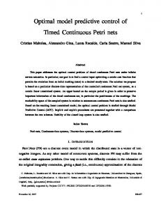
Fig. 9 - IGV Flap Position Response to Feedback Control (a) and to Model Predictive Control (b) To demonstrate the effectiveness of the model predictive optimal control for γ = 1 over the enitre subsonic operating envelope, we compute the control augmentation for all Mach numbers from 0.4 to 0.9. The results are plotted in Fig. 10. As can be seen, the model predictive optimal control is highly effective for all Mach numbers up to 0.8. The Mach number perturbation is well within the tolerance of ±0.001. However, at a Mach number of 0.9, there is a rapid increase in the Mach number perturbation that exceeds the tolerance. The sudden change in the Mach number perturbation at a Mach number of 0.9 is directly attributed to the well-known phenomenon of transonic flow where many linear perturbation theories break down near a Mach number of unity. The term β (x, t) in the linear perturbation model reveals that it becomes undefined for M = 1. Thus, the validity of this model excludes the transonic region near a Mach number of unity.
14 of 16 American Institute of Aeronautics and Astronautics
−3
1
x 10
0.5
0
∆M
−0.5
−1
−1.5 Mach 0.4 @ 310 rpm Mach 0.5 @ 375 rpm Mach 0.6 @ 455 rpm Mach 0.7 @ 455 rpm Mach 0.7 @ 520 rpm Mach 0.8 @ 520 rpm Mach 0.8 @ 590 rpm Mach 0.9 @ 590 rpm Mach 0.9 @645 rpm
−2
−2.5
−3
0
5
10
15 t, sec
20
25
30
Fig. 10 - Test Section Subsonic Mach Number Responses In general, the accuracy of a model predictive control is predicated upon the goodness of the parameter estimation of the disturbance. Any significant deviation from the planned trajectory of the total pressure disturbance will likely cause the Mach number to not meet the required accuracy. Thus, to implement a predictive control scheme, it is necessary to have a priori knowledge of the time variation of the total pressure disturbance as a function of the drag coefficient of the test model. During a pitch polar, the drag coefficient generally varies as a function of the inputs parameters that include the pitch angle, the Mach number, and the Reynolds number. A parameter estimation process can be established using a recursive least-squares or a neural network algorithm to estimate on-line the drag coefficient from the input parameters. In addition, using the knowledge of the time response of the model support system, a trajectory of the total pressure disturbance w (t) can be estimated and used to predict the control augmentation from the math model. Using the predictive results of the control augmentation, the compressor control would be switched to an open-loop mode and begin its actuation simultaneously with the model support system. At the end of the actuation, the compressor control would then be switched back to a feedback mode. Because the control is a feedforward scheme, stability should not be an issue. The model predictive optimal control thus potentially offers a significant advantage over the current feedback control approach which has been demonstrated by simulations and observations to be unable to hold the test section Mach number to within a specified accuracy during a continuous pitch polar of the test model.
VI. Conclusions This paper presents some recent results in optimal control of a distributed-parameter system governed by first order, quasilinear hyperbolic partial differential equations that is controlled by a boundary control process via a periodic boundary condition. The boundary control is further constrained by an ordinary differential equation that models an actuator dynamics that exists at the boundary of the system. The resulting coupled hyperbolic partial-ordinary differential equation system arises in many physical applications involving transport processes such as traffic or fluid flow. Necessary conditions for optimality is derived for this system using the adjoint method which is formulated in terms of dual Hamiltonian functions for the partial differential equation and ordinary differential equation systems. A linear-quadratic optimal control is developed that results in a two-point boundary value problem involving timeshifted solutions due to the periodic boundary condition. By introducing a time horizon parameter, the optimal control problem is found to have a Riccati solution. The results are applied to design a model predictive control for the Mach number in a wind tunnel. A feedback control and and a model predictive control are designed to regulate the test section Mach number due to a total pressure disturbance generated by a test model pitch motion. The feedback control is unable to maintain the test section Mach number to within a prescribed tolerance due to a time delay in the control inputs. In contrast, the model predictive control is shown to be highly effective in maintaining the test section Mach number to within the required accuracy by relying on a model prediction of the control inputs in advance in order to eliminate the time delay effect.
15 of 16 American Institute of Aeronautics and Astronautics
References 1 Debnath,
L., Nonlinear Partial Differential Equations for Scientists and Engineers, Birkhauser, Boston, 1997. B., Frank, H., Rosenbaum, D. M., Steiglitz, K., Kleitman, D. J., “Optimal Design of Offshore Natural-Gas Pipeline Systems”, Journal of the Operations Research Society of America, Vol. 18, No. 6, December 1970, pp. 992-1020. 3 Bayen, A. M., Raffard, R., Tomlin, C. J., “Adjoint-Based Constrained Control of Eulerian Transportation Networks: Application to Air Traffic Control”, Proceeding of the 2004 American Control Conference, June 2004, pp. 5539-5545. 4 Lee, H. Y., Lee, H.-W., Kim, D., “Dynamic States of a Continuum Traffic Equation with On-Ramp”, Physical Review E, Vol. 59, No. 5, May 1999, pp. 5101-5111. 5 J. F. Wendt, Computational Fluid Dynamics - An Introduction, 2nd Edition, Springer-Verlag, 1996. 6 Hou, L. S., and Yan, Y., “Dynamics for Controlled Navier-Stokes Systems with Distributed Controls”, SIAM Journal on Control and Optimization, Vol. 35, No. 2, 1997, pp. 654-677. 7 Nguyen, N., Bright, M., and Culley, D., “Feedback Interior Pointwise Control of Euler Equations for Flow Separation Control in Compressors”, AIAA Flow Control Conference, AIAA-2006-3020, June 2006. 8 Raymond, J. and Zidani, H., “Pontryagin’s Principle for State-Constrained Control Problems Governed by Parabolic Equations with Unbounded Controls”, SIAM Journal on Control and Optimization, Vol. 36, No. 6, 1998, pp. 1853-1879. 9 Casas, E., Tröltzsch, F., and Unger, A., “Second Order Necessary Optimality Conditions for some State Constrained Control Problems of Semilinear Elliptic Equations”, SIAM Journal on Control and Optimization, Vol. 39, 1999, pp. 211-228. 10 Kazemi, M. A., “A Gradient Technique for an Optimal Control Problem Governed by a System of Nonlinear First Order Partial Differential Equations”, Journal of Australian Mathematical Society, Ser. B 36, 1994, 261-273. 11 Jameson, A., Pierce, N., Martinelli, L., “Optimum Aerodynamic Design Using the Navier-Stokes Equations”, Theoretical Computational Fluid Dynamics, Vol. 10, 1998, pp. 213-237. 12 Nadarajah, S., and Jameson, A., “A Comparison of The Continuous and Discrete Adjoint Approach to Automatic Aerodynamic Optimization”, AIAA Conference, AIAA-2000-0667, January 2000. 13 Hirsh, C., Numerical Computation of Internal and External Flows, Vol. 1, John Wiley & Sons, Brussels, 1991. 14 Diller, D., “A Note on the Uniqueness of Entropy Solutions to First Order Quasilinear Equations”, Electronic Journal of Differential Equations, Vol. 1994, No. 5, 1994, pp. 1-4. 15 A. E. Bryson, Jr. and Y. Ho, Applied Optimal Control - Optimization, Estimation, and Control, John Wiley & Sons, New York, 1975. 16 Sagan, H., Introduction to the Calculus of Variations, New York, Dover Publications, Inc., 1992. 2 Rothfarb,
16 of 16 American Institute of Aeronautics and Astronautics