Model Selection Methods for Unidimensional and

Model Selection Methods for Unidimensional and Multidimensional IRT Models

by Taehoon Kang

A dissertation submitted in partial fulfillment of the requirements for the degree of

Doctor of Philosophy (Educational Psychology)

at the University of Wisconsin-Madison 2006

c Copyright by Taehoon Kang 2006

All Rights Reserved

Acknowledgements I would like to gratefully and sincerely thank Dr. Daniel M. Bolt for his guidance, understanding, patience, and most importantly, his friendship during my staying at UW-Madison for six years. His mentorship was paramount and helped me a lot during my PhD study. He encouraged me to not only grow as an psychometrician but also as an independent thinker. He was always available when I needed his help. For everything you’ve done for me, Dr. Bolt, I thank you. I would also like to thank people at T&E services for providing me with a perfect research environment. I am specially grateful to my supervisor, Dr. James A. Wollack. During my project assistantship at T&E, he was always supportive for the progress of my work. Thanks to his thoughtfulness and guidance, I could complete my PhD study in a very warm and safe atmosphere. I would also like to thank Dr. Allan S. Cohen for his assistance and guidance in getting my graduate career started on the right foot and providing me with the foundation for becoming a scholar studying educational measurement. I should say that I was so lucky to be able to meet him as my first advisor in the states. Additionally, I am very grateful for the friendship of all colleagues I have met in Madison, especially Craig Wells, Andrew Mroch, Yanmei Lee, Jianbin Fu, Chanho Park, Hyun-Jung Sung, and Youngsuk Suh. With both personal and academical relationships with them, my life in UW-Madison could be both productive and happy. Finally and most importantly, I would like to thank my wife Minjee. Her support, encouragement, quiet patience and unwavering love were undeniably the bedrock upon which my life have been built. I thank my parents for their endless love, and unconditional help. Also, I thank Minjee’s parents for giving me unending faith and support.

i

Contents List of Tables

iv

List of Figures

vi

Abstract

vii

1 Introduction

1

1.1

Motivation for studying IRT model selection . . . . . . . . . . . . . .

1

1.2

What is the best model? . . . . . . . . . . . . . . . . . . . . . . . . .

2

1.3

IRT model selection for Rasch modelers. . . . . . . . . . . . . . . . .

5

1.4

Research strategy and study overview . . . . . . . . . . . . . . . . . .

7

2 IRT Models and Consequences of Model Misspecification 2.1

2.2

10

Unidimensional and multidimensional IRT models . . . . . . . . . . . 10 2.1.1

Unidimensional dichotomous IRT models . . . . . . . . . . . . 10

2.1.2

Unidimensional polytomous IRT models . . . . . . . . . . . . 16

2.1.3

Exploratory multidimensional IRT models . . . . . . . . . . . 20

Consequences of model misspecification . . . . . . . . . . . . . . . . . 22 2.2.1

Test equating . . . . . . . . . . . . . . . . . . . . . . . . . . . 22

2.2.2

Ability parameter estimation . . . . . . . . . . . . . . . . . . . 23

2.2.3

Computerized adaptive testing (CAT)

2.2.4

DIF analysis . . . . . . . . . . . . . . . . . . . . . . . . . . . . 26

3 Model Selection Methods

. . . . . . . . . . . . . 25

28

3.1

Na¨ıve empiricism . . . . . . . . . . . . . . . . . . . . . . . . . . . . . 28

3.2

LR test

3.3

Information-theoretic methods . . . . . . . . . . . . . . . . . . . . . . 30

3.4

Bayesian methods . . . . . . . . . . . . . . . . . . . . . . . . . . . . . 32

3.5

Cross validation approach . . . . . . . . . . . . . . . . . . . . . . . . 36

. . . . . . . . . . . . . . . . . . . . . . . . . . . . . . . . . . 29

ii 4 Example Studies on Real Data 4.1

4.2

4.3

41

Unidimensional IRT model selection for NAEP data . . . . . . . . . . 41 4.1.1

What is the best dichotomous IRT model? . . . . . . . . . . . 41

4.1.2

What is the best polytomous IRT model? . . . . . . . . . . . 49

Assessing test multidimensionality: Format effects . . . . . . . . . . . 53 4.2.1

Previous studies on format effects . . . . . . . . . . . . . . . . 54

4.2.2

Empirical study on format effects in NAEP data . . . . . . . . 56

Discussion of the example studies . . . . . . . . . . . . . . . . . . . . 62 4.3.1

Noise in the item response data. . . . . . . . . . . . . . . . . . 62

4.3.2

Implication of the example studies

. . . . . . . . . . . . . . . 66

5 Simulation Studies involving IRT Model Selection Methods 5.1

5.2

5.3

68

Study 1: Unidimensional dichotomous IRT models . . . . . . . . . . . 68 5.1.1

Introduction . . . . . . . . . . . . . . . . . . . . . . . . . . . . 68

5.1.2

Simulation study design . . . . . . . . . . . . . . . . . . . . . 69

5.1.3

Simulation study results . . . . . . . . . . . . . . . . . . . . . 70

5.1.4

Discussion of Study 1 . . . . . . . . . . . . . . . . . . . . . . . 80

Study 2: Unidimensional polytomous IRT models . . . . . . . . . . . 83 5.2.1

Introduction . . . . . . . . . . . . . . . . . . . . . . . . . . . . 83

5.2.2


5.2.3


5.2.4


Study 3: Exploratory multidimensional IRT models . . . . . . . . . . 97 5.3.1

Introduction . . . . . . . . . . . . . . . . . . . . . . . . . . . . 97

5.3.2


5.3.3


5.3.4

Nonparametric methods for assessing test dimensionality . . . 109

5.3.5


iii 6 Discussions and Conclusions

118

6.1

Summary recommendations . . . . . . . . . . . . . . . . . . . . . . . 118

6.2

Future directions . . . . . . . . . . . . . . . . . . . . . . . . . . . . . 120

6.3

General summary and conclusions . . . . . . . . . . . . . . . . . . . . 122

Bibliography

125

Appendices A: extra tables

142

Appendices B: computer program codes

174

iv

List of Tables 1

Item Statistics for 1996 State NAEP Math Data . . . . . . . . . . . . 45

2

Comparisons of Model Selection Methods (1996 State NAEP Math Data: block 4 with 21 Multiple-Choice Items) . . . . . . . . . . . . . 47

3

Comparisons of Model Selection Methods (1996 State NAEP Math Data: block 6 with 16 Dichotomous Open-Ended Items) . . . . . . . 49

4

Item statistics for 2000 State NAEP Math Data . . . . . . . . . . . . 53

5

Comparisons of model selection methods (2000 state NAEP math data: 5 polytomous items from block 15)

6

. . . . . . . . . . . . . . . 54

Comparisons of model selection methods (1996 state NAEP math data: Mixed format test with 9 MC and 4 CR items) . . . . . . . . . 62

7

The discrimination parameter estimates of the MIM for the 13 item test: 9 MC and 4 CR items . . . . . . . . . . . . . . . . . . . . . . . 63

8

2 ) Calculated at Item Level for SNR (σT2i /σE2 i ) and Reliability (σT2i /σX i

block 4 and block 6 of 1996 State NAEP Math Data

. . . . . . . . . 65

9

Study 1: Item Parameter Recovery Statistics of the 1PLM: r¯(SD) . . 72

10


11


12

Study 1: Frequencies of correct model selection by conditions (percentage) . . . . . . . . . . . . . . . . . . . . . . . . . . . . . . . . . . 79

13

Study 1: Frequencies of correct model selection by each factor (percentage) . . . . . . . . . . . . . . . . . . . . . . . . . . . . . . . . . . 79

14

Study 1: Model Recovery by CVLL with different kinds of priors . . . 82

15

Study 2: Item Parameter Recovery Statistics of the RSM: r¯(SD) . . . 86

16

Study 2: Item Parameter Recovery Statistics of the PCM: r¯(SD) . . . 86

17

Study 2: Item Parameter Recovery Statistics of the GPCM: r¯(SD) . . 88

18

Study 2: Item Parameter Recovery Statistics of the GRM: r¯(SD) . . . 88

v 19


20


21

Study 2: Type I error Results: GRM-LR and GPCM-LR . . . . . . . 96

22

Latent-Ability Correlation Structures . . . . . . . . . . . . . . . . . . 99

23

Study 3: Item Parameter Recovery Statistics of the 2D-M2PLM: r¯(SD)103

24


25


26


27


28

Study 3: Averages of Simple Matching Similarity Coefficients when Data Were Generated with the M2PLMs . . . . . . . . . . . . . . . . 112

29

Study 3: Frequencies of Clusters’ Numbers, D∗ (P ), and rˆP obtained using DETECT when Data Were Generated with the M2PLMs . . . 114

vi

List of Figures 1

ICCs derived by varying β parameters in the 1PLM . . . . . . . . . . 12

2

ICCs derived by varying α parameters in the 2PLM . . . . . . . . . . 13

3

ICCs derived by varying γ parameters in the 3PLM . . . . . . . . . . 14

4

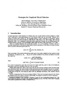
Properties of simple and complex models . . . . . . . . . . . . . . . . 15

5

Category response curves for the example item under the GPCM: α = 1, β = 0, τ 1 = 1.5, τ 2 = 1, τ 3 = 0, and τ 4 = −2.5 . . . . . . . . 17

6

Boundary characteristic curves for the example item under the GRM

7

Category response curves for the example item under the GPCM:

18

α = 1, β = 0, τ 1 = 1.5, τ 2 = 0, τ 3 = 1, and τ 4 = −2.5 . . . . . . . . 20 8

Plots of eigenvalues for block 4 and block 6 data of 1996 NAEP math 44

9

Observed item curve for item 19 in block 4 of 1996 NAEP math . . . 46

10

Observed item curve for item 10 in block 6 of 1996 NAEP math . . . 46

11

The expected and observed raw-score distribution (3PLM) . . . . . . 48

12

Plots of eigenvalues for the 2000 NAEP math test data . . . . . . . . 52

13

(a) UIM as one-factor model and (b) MIM as bifactor model . . . . . 58

14

Trace plots of the αg parameters . . . . . . . . . . . . . . . . . . . . . 61

15

Perfect GOF and good predictive accuracy . . . . . . . . . . . . . . . 62

16

2×2 table to calculate a simple matching similarity coefficient . . . . 111

vii Abstract Item response theory (IRT) consists of a family of mathematical models designed to describe the performance of examinees on test items. Efficient fit of the model to the data is important if the benefits of IRT are to be obtained. Although there is now an extensive research literature on IRT, relatively little has been done to help practitioners evaluate the suitability of specific models for item response data. This study concentrated on issues related to IRT model selection. First, the meaning of model selection is explored emphasizing the principle of parsimony. Next, the importance of model selection in the context of IRT is discussed. After introducing IRT models and problems caused by model misspecification, various model selection methods are investigated. A detailed investigation is provided into several model selection methods, including the likelihood ratio test, information-theoretic methods, Bayesian methods, and new cross-validation approach. The relative success of the indices in choosing the best model among many available unidimensional or multidimensional IRT models is examined. As example studies, applications of model selection methods were performed using real data sets from the 1996 State NAEP mathematics tests for grade 8. First, IRT model selection was used to choose the most appropriate unidimensional IRT model. Second, the multidimensional structure of a mixed format test referred to as a format effect model was investigated through use of model selection indices. The examples illustrate the potential for inconsistency in model selection depending on which of the indices is used. Finally, the model selection methods were compared using simulated data from various unidimensional and multidimensional IRT models. Three simulation studies were conducted for these purposes. The first two studies investigated the IRT model selection methods under conditions of approximate unidimensionality. The first study (Study 1) applied the model selection methods to binary item response data from a test consisting of multiple-choice items or dichotomously scored items.

viii The second study (Study 2) applied methods to a test containing polytomouslyscored items. The last simulation study (Study 3) utilized exploratory multidimensional item response theory (MIRT) models to identify the dimensional structure of test data. In this context, the model selection methods would be applied in an exploratory fashion to sets of dichotomously-scored items of varying dimensionality. The performances of the model selection methods were further compared to nonparametric procedures for dimensionality detection using the same simulated data. Through the simulation studies, in general, two Bayesian model selection methods (DIC and CVLL) appeared to be more stable and accurate in model selection than the other four indices in finding the correct IRT model. The LR, AIC and BIC showed very good performances, but appeared to lack consistency in given conditions. The L50CV did not work well for the purpose of model selection. The DETECT program appeared inferior to the CVLL in evaluating unidimensionality and determining the number of dimensions. These results are encouraging as Bayesian estimation of models is becoming increasingly common.

1

1

Introduction

1.1

Motivation for studying IRT model selection

Model selection is the process by which a specific statistical model is chosen to represent the data. The process has recently become important in item response theory (IRT) due to the introduction of many new and competing models that can be applied to the same type of data. For example, numerous IRT model specifications now exist for characterizing unidimensional item response data from Likerttype scales. Whereas IRT originally embodied only a few well-defined models, it now consists of a broad family of mathematical models including many designed to account for unique features of item response data (e.g., nonmonotonicity, multidimensionality). Selection of an appropriate IRT model is critical if the benefits of IRT for applications such as test development, item banking, differential item functioning (DIF), computerized adaptive testing (CAT), and test equating are to be attained. Consequently, measurement researchers and practitioners often struggle with the question of which IRT model should be applied to their test data. Although there now exists an extensive IRT literature, relatively little has focused on methodology for determining the appropriateness of particular IRT models, and particular model comparison criteria. This has had the unfortunate consequence of many simply choosing a model with which they are familiar or for which software is available (Bolt, 2002; Embretson & Reise, 2000). Because appropriate use of IRT models frequently depends heavily on model fit, the model selection process should be an important part in every application of IRT. If the wrong IRT model is selected for test data, the consequences can be severe in some cases. Yen (1981) explained the possible problems that could be caused by the use of an inappropriate model for dichotomous item response data. Perhaps most critically, the hallmark feature of IRT, parameter invariance, no longer

2 applies (Shepard, Camilli & Williams, 1984; Bolt, 2002; Rupp & Zumbo, 2004). Consequently, item parameters of IRT models became population dependent, and applications of IRT test equating (Bolt, 1999; Camilli, Wang, & Fesq, 1995; Dorans & Kingston, 1985; Kaskowitz & De Ayala, 2001), parameter estimation (DeMars, 2005, Wainer & Thissen, 1987; Walker & Beretvas, 2003; Zenisky, Hambleton & Sireci, 1999), CAT (Ackerman, 1991; De Ayala, Dodd, & Koch, 1992; Greaud-Folk & Green, 1989), person-fit assessment (Drasgow, 1982; Meijer & Sijtsma, 1995), and DIF analysis (Bolt, 2002) can be deleteriously affected. Even beyond the practical implications of choosing an appropriate model, the model selection process can also help clarify the nature of the processes underlying test item responses. Many of the currently proposed IRT models differ according to (1) how they characterize the nature of ability (e.g., unidimensional versus multidimensional) and (2) how they characterize the cognitive mechanisms by which item scores are achieved (e.g., partial credit scoring versus graded response scoring). Because such insights are often a part of test validation, the methods studied in this dissertation may also assist IRT researchers/practitioners in the process of determining whether their tests measure what they are designed to measure.

1.2

What is the best model?

There is no model that can perfectly describe a given set of data, because neither a theory nor a model can be a perfect mirror of reality (Wainer & Thissen, 1987). All that can be achieved is a faithful attempt to find the best model providing a sound connection between theoretical ideas and observed data (Navarro & Myung, 2005). The best model can be defined in different ways depending on the goal of model selection. When the goal of model selection is only to find the model that provides the maximum fit to a given dataset, a model with the smallest root mean squared deviation (RMSD) between the observed and the expected responses may be the

3 best model (Myung & Pitt, 2004). In a similar vein, after calibrating models using a maximum likelihood method, the model with the greatest likelihood may be the best (Akkermans, 1998; Forster, 1986, 2000). But, as Pitt, Kim, and Myung (2003) have noted, the goal of model selection can also be to identify the one model, from a set of competing models, that best captures the regularities or trends underlying the cognitive process of interest. In the context of IRT, for example, if the only feature of interest were item difficulty, a model (such as the two parameter logistic model: 2PLM) which also adds an account of item discrimination might actually confuse understanding of the item characteristic of interest. Forster (2004) named the former approach “na¨ıve empiricism” and warned that it would be problematic because it tends to indicate that the more complex model will be the better model, at least when the models are nested. This approach orients itself towards finding the model that fits the data perfectly. By doing so, the noise (idiosyncratic information) in the data will be fitted at the expense of the signal (structural information) behind the noise. Such “data dredging” may lead researchers to the discovery of spurious effects (Burnham & Anderson, 2002). This is why overfitting is undesirable. As Hitchcock and Sober (2004) indicated, the overfitting is a “sin” when it degrades the predictive accuracy of a theory or model. With an unnecessarily complicated model, therefore, predictions about unseen and future data sets can worsen (Ghosh & Samanta, 2001). A more complicated model than appropriate violates the fundamental scientific principle of parsimony, which requires that one should choose the simplest of all the models that explain the data well. The medieval English philosopher and Franciscan monk, William of Occam, talked about the same principle which came to be known as Occam’s razor. This philosophy implies that “One should not increase, beyond what is necessary, the number of entities required to explain anything (p.1)” (Heylighen, 1997). A model chosen by pursuing this logical principle will have less chance of introducing inconsistencies, ambiguities and redundancies. Similarly, Sir

4 Issac Newton’s first rule of hypothesizing taught us that “we are not to admit any more causes of natural things such as are both true and sufficient to explain their appearance (p.205)” (Forster, 2000). Then, it should be noted that the definition of best involves the principle of parsimony. Geisser and Eddy (1979) wrote, “Which of the models M1 , ..., Mm best explains a given set of data? This is a fundamental question confronting research workers...... While this question is of interest, it is not the crucial one. In most circumstances, a more pertinent one is which of the models M1 , ..., Mm yields the best predictions for future observations from the same process which generated the given set of data? (p.153)” In other words, the aim of model selection is to choose a model that not only provides sound goodness-of-fit (GOF) to the data at hand, but has the ability to generalize to predictions of future or different data. Masters (1982) also emphasized the importance of such generality of item parameter estimates. Indeed, most practical applications of IRT involve the use of item parameter estimates from one test applied to other test forms. It is important to note that a psychometric model captures both structural and idiosyncratic information. The structural information should be as replicable and consistent as possible about the subjects we are interested in, similar to the true score (T ) in the basic formula of classical test theory (CTT). The fundamental principle underlying CTT is captured by the expression, X = T + E,

(1)

where X is the observed total test score of an examinee. The error of measurement, E, is an error term representing the departure of the observed score from true score, and whose standard deviation, σE , is often referred to as the standard error of measurement (Crocker & Algina, 1986). In IRT, a similar representation is defined at the item level (Baker & Kim, 2004; Lord & Novick, 1968). Most IRT models are based on probit (Bock, 1997; Finney, 1952) or logistic (Baker & Kim, 2004; Fisher

5 & Yates, 1938) link functions. Specifically, probit(p) or logit(p) = F (ω) + E,

(2)

where p represents the observed probability of obtaining a category score in an item. Further, ω includes all the item and ability parameter estimates of interest. For each IRT model, the nature of the structural information captured will be different. Consequently, the quality of inference depends on the quality of the chosen model. The best model should extract the relevant structural information from a given dataset as much as possible without loss of predictive accuracy. Such a loss might be caused by idiosyncratic information being explained as structural due to an undesirable high level of model complexity (i.e. the number of parameters). In brief, we want to choose the model that can explain all of the important features of the actual data without adding complexity that is unnecessary. In this dissertation, the likelihood ratio test, information-theoretic methods, Bayesian methods, and a cross-validation approach (all of which will be fully explained later) are used in comparing IRT models, as they are known to be able to consider a model’s complexity as well as its GOF (Akaike, 1974; Forster, 1999; Kadane & Lazar, 2004; Massaro, Cohen, Campbell, & Rodriguez, 2001; Pitt, Kim, & Myung, 2003; Schwarz, 1978).

1.3

IRT model selection for Rasch modelers.

Many IRT modelers, actually, follow a psychometric model tradition established by Rasch (1960/1980). Under this approach, the statistical model for psychologicaltest data is chosen to possess specific measurement properties (Thissen & Orlando, 2001): 1. The desirable properties are defined mathematically. 2. A psychometric model that meets those properties is decided.

6 3. Psychological or educational test data must fit the chosen model. If the basic approach taken in this dissertation were thought of as “Data First”, then the Rasch-based approach would be “Model First”. As Thissen and Orlando (2001) indicated, the difference between the two approaches is more philosophical than caused by any misunderstanding. There have been a few studies (e.g. Hemker et al., 1997; Van der Ark, 2001, 2005) investigating whether various measurement properties could be met by competing IRT models. When Van der Ark (2001) investigated whether various polytomous IRT models could meet measurement properties such as monotonicity (M), monotone likelihood ratio (MLR), stochastic ordering of the manifest variable (SOM), stochastic ordering of the latent trait (SOL), and invariant item ordiering (IIO), only the RSM, which is one of the Rasch models, appeared to satisfy all measurement properties. Samejima (1997) also noted that MLR could be used to indicate how close the model in question is to the Rasch model. According to Wright (1994), “the Rasch model · · · is not designed to fit any data, but instead is derived to define measurement (p. 197)”. Under this approach, the model selection process studied in this dissertation is not necessary and no substantial model evaluation is required. Thissen and Orlando (2001) expressed this approach through the idea that “the item-response model is used as a Procrustean bed (p.90)”. In making model selection decisions, the importance of considering non-statistical issues, including the match of underlying psychological process or measurement properties should not be overlooked. This dissertation was only intended to examine model selection from a model-data fit perspective considering the principle of parsimony. Also, this dissertation is based on the belief that efficient and effective model fit is a paramount consideration in selecting a psychometrical model.

7

1.4

Research strategy and study overview The subsequent chapters will be limited to model selection issues concerning

unidimensional and multidimensional IRT models. The IRT models in this dissertation are all common parametric models. The main interest is on assessing which IRT model is the most appropriate through various model selection methods rather than on deciding whether a specific model fits given data or not. Prior to analyzing the model selection procedures, the unidimensional and multidimensional IRT models to be considered will be reviewed along with the undesirable results caused by model misspecification as indicated by previous research. Next, the available IRT model selection procedures will be summarized with the introduction of recent trials concerning model selection in IRT. As example studies, model selection methods will be applied to real data sets in two studies using 1996 NAEP mathematics test data. • In the first of these studies, IRT model selection will be applied to data from the 1996 and 2000 State NAEP mathematics tests from grade 8. The State NAEP mathematics items were divided into 13 unique blocks. Test booklets were developed for the State NAEP each containing different combinations of three of the 13 blocks. The design of the booklets ensured that each block was administered to a representative sample of students within each jurisdiction. Students were allowed a total of 45 minutes for completion of all three blocks in a booklet. (Allen et al., 1997). IRT model selection for the NAEP data is conducted for two cases: 1) selecting one of the unidimensional dichotomous models for multiple-choice or dichtomously scored items, and 2) selecting one of the unidimensional polytomous models for items with more than two categories. • Second, it is examined whether multiple-choice (MC) and constructed-response (CR) items are measuring the same construct or not on the 1996 NAEP math-

8 ematics tests. A test with items of different formats is commonly called a mixed-format test. When a MIRT model has design structures or mathematical models to link items to specified traits, the model could be considered a confirmatory MIRT model. A kind of confirmatory multidimensionality caused by such different formats is referred to as format effect multidimensionality. Briefly, the model selection indices will be applied to assess format effects in a mixed format test by comparing two models with or without format effects. Finally, three simulation studies will assess the performance of the model selection methods. In each condition, the true model will be one of the compared models. Consequently, it is known which model is the correct model for each generated set of data. • Study 1: The first study will examine the performance of various model selection indices in finding the most appropriate IRT model satisfying both of the GOF and predictive accuracy, when we have binary data sets from a test comprising multiple-choice items or dichotomously scored items. • Study 2: The second study will investigate the performance of a test consisting of polytomously scored items, namely item with more than two score categories. • Study 3: The last simulation study will deal with exploratory MIRT models. In this study, model selection methods will be applied as an exploratory approach to dichotomous data sets that could be of varying dimensionality. Although the most important assumption of IRT is unidimensionality - meaning the domain of items is homogeneous in the sense of measuring a single ability (Baker & Kim, 2004; Embretson & Reise, 2000; Hambleton & Swaminathan, 1985) - two or more abilities may be measured by the test. MIRT models were devised to handle this situation and increase model fit. When test data do

9 not satisfy the assumption of unidimensionality, it is necessary to check if a MIRT model would be more appropriate. Additionally, the performance of the model selection methods will be compared to those of a nonparametric approach in test dimensionality assessment, using the same simulation data sets in Study 3. As Stout et al. (1996) and Tate (2003) indicated, the advantage of a nonparametric method is the fact that it does not depend on a complicated functional form or the strong assumptions which must be satisfied in its parametric counterpart. To evaluate the validity of a model selection approach in assessing multidimensionality, it will be useful to compare these approaches to a non-model-based nonparametric approach such as the DETECT procedure (Kim, 1994) which appeared to have good performance in the detection of test dimensional structure (see Mroch & Bolt, 2006; Tate, 2003; Van Abswoude, Van der Ark & Sijtsma, 2004).

10

2

IRT Models and Consequences of Model Misspecification In this chapter, several IRT models are introduced and consequences of model

misspecification are explored. Thissen and Steinberg (1986) presented a useful taxonomy of item response models that distinguishes models according to several properties. Their taxonomy starts from the set of the simplest models called “Binary Models”, and is extended to three model types; “Left-Side Added Models”, “Difference Models”, and “Divide-By-Total Models”. These distinguishing features, to be described below, also provide a convenient framework for distinguishing the models to be considered in this study.

2.1 2.1.1

Unidimensional and multidimensional IRT models Unidimensional dichotomous IRT models

Although there exist numerous criticisms of multiple choice (MC) items, the efficiency of these items still makes them the typical and most popular item types for large-scale tests. MC items are usually scored 0 for incorrect and 1 for correct, so that an item response dataset generally has as many binary variables as there are items on the test. Thissen and Steinberg’s (1986) taxonomy classifies some IRT models designed to analyze such test items as “Binary Models”. The one-parameter logistic model (1PLM) and 2PLM belong to this set. Suppose Xij represents the response of person j to item i, where Xij = 1 means the item i is answered correctly and Xij = 0 means the item i is answered incorrectly. Then, these two models are expressed as the Equations (3) and (4), respectively.

P (Xij = 1|θj , βi ) =

exp(θj − βi ) , 1 + exp(θj − βi )

(3)

11 P (Xij = 1|θj , αi , βi ) =

exp[αi (θj − βi )] 1 + exp[αi (θj − βi )]

(4)

where θj represents the ability parameter for examinee j; αi (item discrimination) and βi (item difficulty) refer to the parameters of item i. For the 1PLM and 2PLM, βi is the point on the ability (θ) scale at which an examinee has a 50% probability of correctly answering item i. Items with high values of β are difficult items, implying low-ability examinees have low probabilities of correctly responding. Items with low values of β are easy items, implying most examinees, even those with low-ability values, have moderate to high probabilities of answering the item correctly. Theoretically, difficulty values can range from −∞ to +∞; in practice, values usually are in the range of −3 to +3. The discrimination parameter of item i, αi allows the items to differentially discriminate among examinees. Technically, αi is defined as the slope of the item characteristic curve (ICC) at the point of inflection (Baker & Kim, 2004). The α parameter can range in value from −∞ to +∞, with typical values being from 0 to 2. The higher the α value, the more sharply the item discriminates between examinees at the point of inflection. The various ICCs by each model are illustrated in Figures 1 and 2. These two models are distinguished by the existence of a restriction on the item discrimination parameter, α. The 1PLM assumes that all items in a test are equally discriminating, whereas the 2PLM allows items to have different discrimination parameters. Hambleton, Swaminathan, and Rogers (1991) said that the appropriateness of this kind of restrictive assumption depends on the nature of the data and the importance of the intended application. For example, if a criterion-referenced test following effective instruction is relatively easy and constructed from a homogeneous item bank, then the equal-discrimination assumption for the 1PLM may be quite acceptable. On the other hand, if the 1PLM is used for a dataset without such conforming nature, it may result in model misspecification. One of the goals of IRT expressed by Lord (1980) is to have the capacity to predict the performance of any examinee on any item even though the examinee

12 1

probability to answer an item correctly

0.9 0.8 0.7 0.6 0.5 0.4 0.3

beta = - 1 beta = 0 beta= 1

0.2 0.1 0

-3

-2

-1

0

ability (theta scale)

1

2

3

Figure 1: ICCs derived by varying β parameters in the 1PLM may have never taken the item before. The use of a wrong model could harm not only such prediction accuracy but also all the subsequent activities based on IRT. For instance, scaling or equating is one of the most important IRT applications. When it is desired to obtain the comparability of test scores across different tests measuring the same ability, IRT can solve this problem by putting item parameters from different tests on a common scale by using the linear relationship in Equation (5). βX = AβY + K

(5)

αX = αY /A where βX and αX are the difficulty and discrimination parameter estimates in test X, and βY and αY are the corresponding values in test Y. Once scaling constants, A and K, are determined using common items in test X and Y, the item parameters estimates in test Y may be placed on the same scale as the item parameter estimates for test X. Then, the θ estimates in test Y may be placed on the same scale as those

13 1


0.9

0.8

0.7

0.6

0.5

0.4

0.3

alpha=0.5, beta=0 alpha=1.0, beta=0 alpha=1.5, beta=0

0.2

0.1

0

-3

-2

-1

0

1

2

3


Figure 2: ICCs derived by varying α parameters in the 2PLM taking test X by ∗ θX = AθY + K.

(6)

Many linking designs and methods to determine the scaling constants have been devised. Regardless of how elaborative they are, however, using a wrong model may hurt the whole scaling or linking process from the beginning. For example, the A scaling constant should be fixed at 1 for a particular testing program under the 1PLM. If, however, the true model for a given dataset were actually the 2PLM, the actual A would often not be equal to unity. Therefore, equating results based on the 1PLM may not be trustworthy. As Camilli et al. (1995) emphasized, the question “Which calibration model?” should be contemplated before asking “Which equating method?” Within the taxonomy, “Binary models” can be extended to more complex models in one of three directions. One direction leads to “Left-Side Added Models”: An ICC displays the probability of correct response as a function of examinees’ ability (θ), and is usually increasing in θ. Even at very low levels of θ, there may exist a

14 nonzero probability of answering the item correctly. A model that incorporates this nonzero lower asymptote is the three parameter logistic model (3PLM) given by

P (Xij = 1|θj , αi , βi , γi ) = γi + (1 − γi )

exp[αi (θj − βi )] , 1 + exp[αi (θj − βi )]

(7)

where γi refers to the lower asymptote of item i’s ICC. γi is often referred to as the pseudo-guessing parameter, which accounts for the possibility that all examinees, even ones with very low ability, have a nonzero probability of answering multiplechoice items correctly by guessing (Hambleton & Swaminathan, 1985). Theoretically, γ could range from 0 to 1, but typically lies between 0 and 0.3. For the 3PLM, βi is defined as the point at which the probability of correctly answering an item is (1 + γi )/2. The various ICCs with different γi values are illustrated in Figure 3. 1


0.9

0.8

0.7

0.6

0.5

0.4

alpha=1,beta=0,gamma=0.3 alpha=1,beta=0,gamma=0.15 alpha=1,beta=0,gamma=0

0.3

0.2

0.1

0

-3

-2

-1

0

1

2

3


Figure 3: ICCs derived by varying γ parameters in the 3PLM The three models, the 1PLM, 2PLM, and 3PLM, are the most popular IRT models for dichotomous data. All three share two common assumptions. The first assumption is the presence of a single underlying ability, usually a continuous, unbounded variable designated as θ. This assumption is commonly called the assump-

15 tion of unidimensionality. The second assumption, local independence, implies that any 2 items should be statistically independent after controlling for θ. Given ability, performances for all pairs of items are assumed to be locally independent. When γi is set equal to 0 for an item, Equation (7) simplifies to the 2PLM. Furthermore, constraining αi to be equal for all items produces the 1PLM. Thus, the three models share a nested relationship. The three logistic models differ only in terms of the number of parameters used to characterize the item response process.

Simple

Complex

-Fewer parameters -More constraints -Parsimony -Generalizability -e.g. 1PLM

-More parameters -Fewer constraints -Goodness of fit -Flexibility -e.g. 3PLM

Figure 4: Properties of simple and complex models Figure 4 illustrates the main properties of simple and complex models. A model with so many related parameters may explain idiosyncracies (i.e. noise) as well as regularities. It should be noted that the more complicated model always has the fewer constraints imposed (Myung, Pitt, Zhang, & Balasubramanian, 2001). A model with many parameters has greater flexibility to fit diverse patterns of data. Because of the greater relative complexity of the 3PLM, therefore, this model tends to have better GOF than the 1PLM and 2PLM. If the 1PLM and 2PLM are not able to provide satisfactory model fit, the 3PLM may be one of the alternatives chosen. If the extra complexity is unnecessary, however, the 3PLM may lose predictive accuracy for future data sets because the 3PLM is less parsimonious than the 1PLM and 2PLM. In this dissertation, it is assumed that “simple models should be preferred to more complicated ones, other things being equal (p.141)” (Kieseppä, 2001).

16 Within the context of many testing programs, particularly those using computerized adaptive testing (CAT) or computer based testing (CBT), it is very common to use preequating. In preequating, the item parameters should be calibrated and linked on the common scale of those in a preestablished item bank before being administered as operational test forms (Du, Lipkins, & Jones, 2002; Wainer & Mislevy, 2000; Weiss, 1982; Weiss & Kingsbury, 1984). The lack of generalizability or prediction accuracy due to the use of too complex a model may cause severe misfit in this context. 2.1.2

Unidimensional polytomous IRT models

As generalizations of dichotomous IRT models, polytomous IRT models are suitable for items scored using more than two score categories. Many measurement instruments for educational and psychological testing use items with multiple ordered-response categories; such as when partial credit is to be awarded for a partially correct answer. There are many reasons why this format may be preferred. One is the fact this type of scoring is usually more informative and reliable than dichotomous scoring. In this study, we deal with four commonly used polytomous IRT models: the rating scale model (RSM; Andrich, 1978), the partial credit model (PCM; Masters, 1982), the generalized partial credit model (GPCM; Muraki, 1992), and the graded response model (GRM; Samejima, 1969). The first three models, the RSM, PCM, and GPCM, are hierarchically related, and represent a second extension of “Binary Models” in the Thissen and Steinberg (1986) taxonomy, referred to as “Divide-By-Total Models”. The most general of these three models is the GPCM. The probability that an examinee j scores in category x on item i is modeled by the GPCM as P exp xk=0 αi [θj − (βi − τki )] Py P (Xij = x|θj , αi , βi , τki ) = Pm , y=0 exp k=0 αi [θj − (βi − τki )]

(8)

where j = 1, . . . , N , i = 1, . . . , T , and x = 0, . . . , m. In this model, αi represents the discrimination of item i, βi represents the difficulty of item i, and τk represents

17 a location parameter for category k on item i. We set τ0i = 0 and exp (βi − τk )] = 1 in Equation (8) for identification.

P0

k=0

αi [θj −

If the αi is fixed at 1 across items, Equation (8) reduces to the PCM. In addition, if τ values are the same for each category, respectively, across items, Equation (8) further reduces to the RSM. Consequently, like the 1PLM, 2PLM and 3PLM, the RSM, PCM, and GPCM are nested models. Figure 5 shows example category response curves of a polytomous item with five categories (0, 1, 2, 3, and 4) under the GPCM. βi − τ1 through βi − τ4 indicate the locations at which the category response curves intersect on the latent-trait scale. 0.9

alpha=1,beta=0,tau1=1.5,tau2=1,tau3=0,tau4=-2.5

0.8

0.7

4

0 3

probability

0.6

0.5 2 0.4

1

0.3

0.2

0.1

0

-3

-2

-1

0

1

2

3


Figure 5: Category response curves for the example item under the GPCM: α = 1, β = 0, τ 1 = 1.5, τ 2 = 1, τ 3 = 0, and τ 4 = −2.5 The GRM, however, is not a “Divide-By-Total” Model. Instead, the GRM is a representative model of a third extension (“Difference Models”) of Thissen and Steinberg’s taxonomy. It can be viewed as a generalization of the 2PLM that uses the 2PL to model boundary characteristic curves, namely curves that represent the probability of a response higher than a given category x. It is convenient in the model to convert the x = 0, . . . , m category scores into x = 1, . . . , m + 1 categories.

18 ∗ If we use Pijx to denote the boundary probability for examinee j to have a category

score larger than x on item i, then the boundary curve is given by

∗ Pijx =

exp[αi (θj − βxi )] . 1 + exp[αi (θj − βxi )]

(9)

Figure 6 shows example boundary characteristic curves for a five-category item (1, 2, 3, 4, and 5) under the GRM. Note that an item with m + 1 categories results in m boundary curves. 1

0.9

P1 alpha=1, beta1=-1,beta2=-0.5,beta3=0.5,beta4=1.5

0.8 P2 0.7

Probability

P*1

P*2

0.6

P*3

P*4

P3

0.5

0.4 P4 0.3

0.2 P5

0.1

0

-3

-2

-1

0

1

2

3


Figure 6: Boundary characteristic curves for the example item under the GRM To determine the probability of a particular item score, the difference between adjacent categories is used. Thus, in the GRM, the probability that examinee j achieves category score x on item i is given by ∗ ∗ − Pijx Pijx = Pij(x−1)

(10)

∗ ∗ where x = 1, . . . , m + 1, Pij0 = 1, and Pij(m+1) = 0.

As an example, the values of Pij1 through Pij5 when the ability of examinee j is θ = 0.4 is illustrated in Figure 6 as the length of vertical line divided by boundary characteristic curves at the θ = 0.4.

19 The GRM is distinguished from the GPCM and its nested models (the RSM, and PCM) by the fact that it requires a two-step process to compute the conditional probability for an examinee responding in a particular category. As a result, it is referred to as “indirect(p.97)” IRT model by Embretson and Reise (2000). As Myung, Pitt, Zhang, and Balasubramanian (2001) explained, there are at least two independent dimensions of model complexity: the number of free parameters of a model and its functional form (see y = θx and y = xθ ). Even though the GRM and GPCM need the same number of parameters for fitting each item, it should not be said that they have the same model complexity because the functional forms of the models are very different. Furthermore, the scoring process assumed by the GRM (grade response scoring) is conceptually different from that supposed by the PCM and GPCM (partial credit scoring). The former uses 2PLMs to compute boundary curves for each item, so each curve represents the probability of an examinee’s raw item score (x) falling above a given category threshold as shown in Figure 6. (In fact, the βxi s in Equation (9) are often referred to as threshold parameters.) The order of the category thresholds should be kept the same within each item (Samejima, 1969). In partial credit scoring, however, the focus is on the relative difficulty of each step needed to transition from one category to the next in an item. (Therefore, the βi − τki s in Equation (8) are commonly referred to as step parameters.) Within an item, some steps (category intersection) may be relatively easier or more difficult than others. Thus, the property of ordered location parameters is not indispensable. An example is illustrated in Figure 7 . There, the step from x = 1 to x = 2 (step parameter=0) is more difficult to achieve than that from x = 2 to x = 3 (step parameter=-1). The assumed scoring process for the RSM is differentiated from the PCM and GPCM in that the RSM model restricts such step processes to be same across all items in a test. It is often not clear to researchers and practitioners which of the polytomous IRT models provides the best description of the underlying item response process

20 0.7

alpha=1,beta=0,tau1=1.5,tau2=0,tau3=1,tau4= -2.5 0.6 4 0

probability

0.5

3

0.4 1 0.3

2

0.2

0.1

0

-3

-2

-1

0

1

2

3


Figure 7: Category response curves for the example item under the GPCM: α = 1, β = 0, τ 1 = 1.5, τ 2 = 0, τ 3 = 1, and τ 4 = −2.5 for a given set of data (Bolt, 2002). Therefore, techniques for distinguishing between these models are seemingly important, as is research on the benefits of choosing the best model and the resultant problems from choosing a poor model. 2.1.3

Exploratory multidimensional IRT models

As noted previously, the IRT models used in most current applications require that a test be unidimensional. Most educational and psychological tests, however, are multidimensional to some degree (Ackerman, 1994, 1996; Luecht & Miller, 1992; Reckase, 1979, 1997; Traub, 1983). Thus, applications of IRT models require inspection of test data dimensionality (De Ayala & Hertzog, 1991). When it is necessary or desirable to account for such multidimensionality, MIRT models should be applied. MIRT models are generalizations of unidimensional models that add additional trait or ability parameters. Often these multiple traits or abilities can be aligned with specific problem types. An example of a such case is an algebra exam with two basic types of problems: items that require direct solving of algebraic equations

21 (abstract) and items embedded in a problem solving context (word problems). The former item may require algebraic symbol manipulation, while the latter item would additionally require reading comprehension (Ackerman, 1994). MIRT models use two or more trait parameters to represent each examinee. An exploratory MIRT involves estimating item parameters in such a way that permits identification or interpretation of the underlying dimensions. Modeling data in this multidimensional manner also allows separate inferences to be made about the trait levels of an examinee for each distinct dimension being measured (Walker & Berevtas, 2000). If we extend the 2PLM as a multidimensional model, a distinct discrimination parameter can be attached to each dimension for a given item (Bolt & Lall, 2003; Embretson & Reise, 2000; Reckase, 1985, 1997), as follows: P exp( K k=1 αik θjk + δi ) P (Xi = 1|θ, α, δ) = , P 1 + exp( K k=1 αik θjk + δi )

(11)

where θ1 ,...,θK represents K examinee latent traits or abilities, α1 ,..., αK are the trait-specific discrimination parameters, and δi is a multidimensional easiness parameter. If δi is positive and large, thus implies that item i is easy. The model in Equation (11) is referred to as the compensatory multidimensional two-parameter logistic model (M2PLM). The term “compensatory” implies that being low on one trait can be compensated for by higher levels on another trait. For example, two abilities such as reading and language mechanics on a language placement exam might compensate for each other. Compensation occurs because the trait terms are additive in the logit in Equation (11). Research has shown that when data known to be multidimensional are modeled with a unidimensional model, there may be incorrect inferences about characteristics of the items (e.g., discriminations) as well as about a student’s proficiency (Ackerman, 1991; DeMars, 2005; Reckase & McKinley, 1991; Stocking & Eignor, 1986; Walker & Berevtas, 2000). Bolt (1999) and Camilli et al. (1995) discussed

22 the potential problem of unidimensional IRT true-score equating under conditions of test multidimensionality. Also, various studies explained the implication of multidimensionality on DIF (Ackerman, 1992; Roussos & Stout, 1995; Shealy & Stout, 1993). A main purposes of in MIRT is to define the structure of test dimensionality: The number of factors and related loading values should be obtained, followed by the appropriate interpretation of each factor. Many parametric and nonparametric methods for assessing the dimensionality of the latent space underlying responses to test items have been developed (see Tate, 2003; Van Abswoude, Van der Ark, & Sijtsma, 2004). In this dissertation, various model selection methods are examined with respect to their capacity to assess the structure of test dimensionality.

2.2 2.2.1

Consequences of model misspecification Test equating

As Kolen and Brennan (2004) describe, equating is a statistical process used to adjust scores on test forms so that the forms can be used interchangeably. IRT can place different test forms on a common scale of measurement through linking. Scores indicating common levels of examinee ability can then be equated using Equation (6). When an anchor-test design, where each form has a set of common items, is used to obtain linking constants, A and K, the parameters of items embedded in both tests should first be estimated separately. Then, given the separate estimates, we can use one of a variety of methods to estimate optimal A and K values (e.g., regression method, mean/sigma method, mean/mean method, and characteristic curve method) (Hambleton & Swaminathan, 1985, 1991). As Hambleton and Rovinelli (1986) note, the choice of item response model is one of the most important elements in determining the degree of success of a test equating. Naturally, the most appropriate model for equating multiple test forms may be different for different test forms. For example, Kolen (1981) found that

23 the 3PLM was better for equating than the 1PLM in a variety of multiple-choice testing situations. He explained the lack of a guessing parameter in the 1PLM as a possible reason for its poor performance. By contrast, Du, Lipkins, and Jones (2002) compared three dichotomous IRT models for the equating of a national licensing examination and found that the use of the 1PLM was supported by their studies on real and simulated data. They found the equating results for the 2PLM and 3PLM to be unstable especially when the sample size was 500 or smaller. Test multidimensionality has been identified as one of the other threatening factors that can hurt the IRT equating process (Kolen & Harris, 1990; Hendrickson & Kolen, 1999). Dorans and Kingston (1985) and Camilli et al. (1995) investigated the effect of multidimensionality on IRT true-score equating. Through factor analysis, they divided items in a test into homogeneous subgroups, and compared the equating results from a single calibration of the whole test with that from separate calibrations of dimensionally homogeneous item groups. In both studies, they did not find any meaningful differences between the two approaches. Camilli et al. (1995) noted, however, that the high correlation (.7) of the two latent traits measured by the Law School Admission Test (LSAT) might be the cause of these results. In other words, as the correlation between two abilities goes down and the dimensions become more distinct, the quality of equating with the single calibration might worsen. This supposition was assessed and affirmed by Bolt (1999) through a simulation study. When the correlation between two dimensions is high (≥ .7) the unidimensional IRT true-score equating performed at least as well as the traditional equipercentile equating, but when the correlation is moderate to low (≤ .5), the unidimensional IRT true-score equating was found to be inferior to the equipercentile method. 2.2.2

Ability parameter estimation

Jones, Wainer, and Kaplan (1984) showed that error in ability estimates could increase when the chosen test model did not fit the data. After emphasizing the im-

24 portant fact that every IRT model is in truth a simplification of reality, Wainer and Thissen (1987) demonstrated which model among three dichotomous IRT models best fit and provided the most accurate ability estimation when applied to simulated data which were generated from an alternative IRT model. They found that it was clear which model performed poorest, and concluded that accurate ability estimation could be obtained only through a careful combination of the model selection and estimation algorithm. If a wrong model is chosen for the analysis of high-stakes test data, in particular, there may be a fatal error in decision-making for a student. For example, Kalohn and Spray (1999) showed very high classification errors (pass versus fail) were made through incorrect use of the 1PLM when the 3PLM was the true model. There are many studies that have shown that ignoring primary IRT assumptions such as local independence could hurt test reliability and validity, as well as item and ability statistics (For example, Keller, 2003; Sireci, Thissen, & Wainer, 1991; Wainer & Thissen, 1996; Zenisky, Hambleton & Sireci, 1999). Through such studies, it has been shown that the presence of local item dependence (LID) has a significant impact on ability estimation. According to Braeken, Tuerlinckx, and De Boeck (2005), two main problems caused by LID are non-reproducibility and the impossibility of interpreting item parameters. To overcome the problems due to the presence of LID in passage-based or testlet-based tests, modified IRT models have been suggested (i.e., Bradlow, Wainer & Wang, 1999; Du, 1998). A few studies have demonstrated what happens if a unidimensional model is used when a test has items known to be multidimensional. Walker and Beretvas (2003) demonstrated clear differences between unidimensional and two-dimensional confirmatory models in proficiency classification. When a test actually measured two abilities (i.e., ‘general mathematical ability’ and ‘communication ability in mathematics’), multidimensional modeling enabled one to make separate inferences for each of the two dimensions. But, the wrong application of a unidimensional model

25 obstructed valid inferences about students’ math abilities. Because the unidimensional modeling must have provided a single ability estimate that is a type of composite of multidimensioinal abilities, it was not surprising that the inference about student proficiency based on that composite had been different from that provided by a multidimensional model. DeMars (2005) studied scoring methods when a test comprises multiple subtests. The performance of a unidimensional approach was contrasted against various scoring methods that accounted for the multidimensionality, such as bi-factor modeling (Gibbons & Hedeker, 1992), compensatory MIRT modeling and augmented scoring (Wainer et al, 2001). The unidimensional scoring appeared to have greater bias and higher RMSEs in her simulation study. 2.2.3

Computerized adaptive testing (CAT)

The goal of adaptive testing is to provide each examinee with a “tailored” test best matching his or her ability level. In general, adaptive testing without some form of IRT and a powerful computer is not feasible, although some attempts have been made (Hambleton et al., 1991; Weiss, 1982). Wainer et al. (2000) warned that there could be actual differences between the view of human abilities implicit in IRT and that of cognitive and educational psychology. To ensure the valid use of latent trait estimates under the chosen IRT model, therefore, great care should be taken in selecting an appropriate model to use in CAT. De Ayala, Dodd, and Koch (1992) compared the PCM and the GRM under CAT when a test includes items that did not fit these models. They used a linear factor analytic model to generate misfitting items. The GRM-CAT appeared robust to this kind of misfit for ability estimation. The same could not be said for the PCM-CAT, where the more misfitting items the item pool contained the less accurate the ability estimation was. An important and alternative cause of misfit may be due to multidimensionality, an issue not considered in the De Ayala et al. (1992) study. Ackerman (1991)

26 examined the effect of multidimensionality on CAT when all items were assumed unidimensional. According to Ackerman, if some items actually measured two latent traits whose composite was similar to the single ability calibrated with a unidimensional model, the estimated discrimination values for these items tended to be larger than those of items measuring only one of the two traits. Therefore, the multidimensional items were generally more informative and hence more likely to be selected for the CAT administration. Wainer and Mislevy (2000) also warned that serious problems such as poor ability estimation might occur under the incorrect assumption of unidimensionality in CAT, especially when the composite of ability dimensions required to solve an item is radically different across items. On that basis, it is important to have procedures available to identify whether data are better fitted by unidimensional or multidimensional IRT models. 2.2.4

DIF analysis

Since the civil rights era, test fairness has come to be a central issue in psychometrics (Cole, 1993). The term, differential item functioning (DIF), has come to be used to commonly describe empirical evidence of item bias in a technical and neutral way. By definition, DIF occurs when “individuals having the same ability, but from different groups, do not have the same probability of getting the item right (p.110)” (Hambleton et al., 1991). Bolt (2002) provided an illustration that demonstrated the necessity of selecting polytomous IRT models carefully in DIF analysis. To investigate the implication of model misspecification on DIF detection in polytomous response data, he conducted a simulation study to investigate the performances of the LR test under the GRM (referred to as GRM-LR test). Even though the GPCM and GRM appeared to provide similar GOF for a given dataset, model misspecification had more serious implications for DIF analysis. When the best model for a given dataset was the GPCM, but the GRM was used for model calibration and DIF detection, the GRM-

27 LR test suffered from serious Type-I error inflation which would have been controlled if the correct model, the GPCM, were used. The causes of DIF can be attributed to various characteristics of examinees, such as different educational backgrounds, test-taking strategies or varying degrees of motivation among the groups of interest. They can also be attributed to various characteristics of items, and the skills or traits they measure. Such sources can be presumed as either categorical or continuous variables. When they are not intended to be measured, they are sometimes called nuisance dimensions(s) because they serve only to introduce noise to the primary dimension(s) of interest (Roussos & Stout, 1995). Oshima and Miller (1992) showed that the observed DIF can be linked to content dimensions by conducting a simulation study where most of the items in a test were related to only one trait but a portion of the item responses was governed by both the primary trait and a nuisance trait. In this case, without knowing the structure of test multidimensionality, the detection and explanation of DIF might be very difficult. An understanding of the dimensional structure of a test, therefore, is important as a premise for conducting valid and meaningful DIF analyses.

28

3

Model Selection Methods In this section, several available IRT model selection methods are described.

After talking a philosophy of “na¨ıve empiricism”, the likelihood ratio (LR) test is then presented as a method for statistically testing differences in model fit. Next, information-based indices that simultaneously consider model-data fit and complexity are described. Due to the recent appeal of Bayesian methods in IRT estimation, several criteria will be introduced for cases in which a Markov chain Monte Carlo (MCMC) algorithm is used for model calibration. Finally, a cross validation approach using number-correct score distributions is proposed. This method shares a similar mechanism with the well known leave-one-out cross validation approach that underlies more general statistical model selection procedures.

3.1

Na¨ıve empiricism

When the goal of IRT model selection is only to choose the model giving the maximum GOF among several available models, there are several possible procedures. Traditionally, IRT researchers have used criteria such as residual plots (Hambleton et al., 1991) to identify model misfit at the item level. Such criteria provide a way of evaluating the absolute fit of the model to the data, and thus can also be used for model comparison purposes. To apply the na¨ıve empiricism approach to the entire dataset, as Thissen & Orlando (2001) indicated, the root mean squared deviation (RMSD) may be calculated between the expected and the observed examinee raw-score frequency distribution (Kolen, Zeng, & Hanson, 1996; Lord & Wingersky, 1984). Alternatively, when a maximum likelihood method is used for the purpose of calibration, the model with the greatest likelihood can be selected as the best (Akkermans, 1998; Forster, 1986, 2000). In other words, the maximized likelihood value of each competing model can be used as a measure of the model’s GOF (Myung & Pitt, 2004). Because these methods consider only GOF without accounting for

29 parsimony, no model selection indices based on the na¨ıve empiricism approach will be considered in the subsequent sections.

3.2

LR test

When IRT models are nested, it becomes possible to select the better model using a likelihood ratio (LR) test. The LR test statistic, G2 , is a chi-square (χ2 ) based statistic and is calculated as the difference between deviances of the two models being compared. The deviance is defined as −2×log (maximum likelihood). The smaller the deviance for a model, the better fitting the model. The difference is distributed as a chi-square (with degrees of freedom equal to the difference in the numbers of estimated parameters) under a null hypothesis of no difference in model fit between the two models. Therefore, G2 may be tested through a significance test to determine if the more complex model provides a significantly better fit (Anderson, 1973; Baker & Kim, 2004; Bock & Aitkin, 1981; Lierberman, 1970, Reise, Widaman & Pugh, 1993). Even though there is some improvement in fitting with the more complex model, unless it is a substantial enough difference (i.e., statistically significant), the simpler model will be preferred by the LR test. To perform an LR test, the simpler or less parameterized model is usually assumed under the null hypothesis and the more complex model is posited under the alternative hypothesis. To apply the LR test to select one of the three nested dichotomous IRT models (the 1PLM, 2PLM and 3PLM), the deviance statistics provided by the program, BILOG (Mislevy & Bock, 1990), are useful. The null hypothesis, H0 : αi is fixed across all items, can be tested to compare the 1PLM and 2PLM, and the other hypothesis, H0 : γi = 0 across all items, is available to compare the 2PLM and the 3PLM. For the three nested polytomous models (the RSM, PCM, and GPCM), the deviance values calculated by the program, PARSCALE (Muraki & Bock, 1998) can be utilized. For the PCM and GPCM, the same null hypothesis as that used to compare the 1PLM and 2PLM should be used. And, for

30 the RSM and PCM, it can be tested whether or not a set of step parameters is the same across items. Deviance statistics from TESTFACT (Wilson, Woods, & Gibbons,1984) can be used for checking test dimensionality through the LR test. First, one-factor and two-factor models can be compared. The difference in deviances can be regarded as a χ2 variable with degrees of freedom equal to the difference across models in the number of parameters. If the fit improvement is not statistically significant, the assumption of unidimensionality is retained. If the significance test returns a significant result, then the more complicated model, the two-factor model, would be chosen. Thus, the assumption of unidimensionality would be rejected. Models with more than two factors could be tested in a similar way until the LR test result is not significant.

3.3

Information-theoretic methods

Information-based indices are popular in many research areas because they strike a balance between the improvement in model fit and the elegance and predictability of a more parsimonious model (De Boeck, Wilson, & Acton, 2005). According to Sober (2002), Akaike’s framework portrays the model selection problem as one of predictive accuracy. Therefore, it becomes possible to pursue the best model under parsimony considerations using observable evidence. While the LR test is only applicable when comparing models that are nested, information criteria such as Akaike’s information criterion (AIC: Akaike, 1974) or Schwarz’s Bayesian information criterion (BIC: Schwarz, 1978) may be used to compare models regardless of whether or not the models are nested (Burnham & Anderson, 2002; Sober, 2002). Although significance tests are not possible with these statistics, they do provide estimates of the relative differences between solutions. The AIC has components representing GOF and complexity. The first component is the deviance (d) defined above. The second component is 2 × p, where p is

31 the number of estimated parameters, which can be interpreted as a penalty function for over-parameterization. This penalty is designed to correct for overfitting. The AIC is thus defined as: AIC(M odel) = d + 2p.

(12)

The model with the smallest AIC is the one to be selected. If a simple and a complex model fit a dataset equally well, the simpler model will have the smaller AIC (Hitchcock & Sober, 2004). A criticism of the AIC is that it is not asymptotically consistent because sample size is not directly involved in its calculation (Ostini & Nering, 2005; Schwarz, 1978; Sclove, 1987). When applied to data with large N , according to Forster (2004), this method tends to provide similar model selection results to that of na¨ıve empiricism. Consequently, the AIC tends to prefer saturated models in very large samples (Janssen & De Boeck, 1999). An alternate criterion similar to the AIC is the BIC. These two indices represent the most popular information criteria for statistical model selection (Kieseppä, 2001). Schwarz (1978) developed the model selection measure, BIC, based on a Bayesian argument. The BIC achieves asymptotic consistency by penalizing overparameterization through the use of a logarithmic function of the sample size. The BIC criterion is defined as BIC(M odel) = d + p · (logN ),

(13)

where N is the sample size. Whereas AIC multiplies p by a constant 2, p is multiplied by a number proportional to the sample size, which is the natural logarithm of N . Therefore, with the BIC, the penalty for increasing the number of parameters is more severe, particularly for data sets with large N . Not surprisingly, BIC tends to favor simper models relative to the AIC, when the sample size is large. As Lin & Dayton (1997) and Lubke & Muthén (2005) have noted, results from these two statistics do not always agree with each other because they have different penalties on the number of parameters.

32 When a psychometrician builds a new psychometric model as an extension of an already-established model or wants to choose one among several candidate models to apply to a given dataset, a comparison between models is needed. In this kind of situation, the information criteria have been widely used. Many examples of applications of information criteria in IRT contexts exist (see San Martin, Del Pino, & De Boeck, 2005; Wilson, 1992; Wilson & Adams, 1993, 1995). Such studies seek to find the most acceptable and appropriate models for given sets of real data, using AIC or BIC. Also, to deal with the multidimensional latent space associated with a test, some studies have tried to evaluate test dimensionality based on substantive theory. The information criteria have been used to compare multiple models having different numbers of dimensions and being built from different cognitive theories (see Janssen & De Boeck, 1999; McMahon & Harvey, 2005). There are two issues to be noted about the use of information criteria. First, it is usually not known which of these criteria provides the best results in specific cases (Wagner & Timmer, 2001). Second, it is not always guaranteed that the criteria are appropriate for comparing non-nested models with different types of parameters or scales (Hong & Preston, 2005; Ostini & Nering, 2005). In spite of such common uses of these information criteria, their performances in IRT applications have not been investigated systematically. Therefore, one of the goals of this dissertation is to investigate the performances of information-based indices in an IRT context through simulation studies.

3.4

Bayesian methods

AIC and BIC are available whenever maximum likelihood estimates of model parameters are obtained. As Lin and Dayton (1997), Lord (1975), and Sahu (2002) note, however, asymptotic estimates of item parameters are not always available. When such is the case, neither AIC nor BIC are appropriate. For such situations, Bayesian parameter estimation is sometimes an effective alternative. Such estimates

33 are obtained, for example, when using Markov chain Monte Carlo (MCMC) methods. Two Bayesian model selection methods that have been suggested when MCMC methods are used for estimation of IRT model parameters are the pseudo-Bayes factor (PsBF: Bolt, Cohen & Wollack, 2001; Geisser & Eddy, 1979; Gelfand & Dey, 1994; Sahu, 2002), and the Deviance Information Criterion (DIC: Spiegelhalter, Best, & Carlin, 1998). I describe these methods next. A common Bayesian approach to comparing two models, say a Model A and a Model B, is to compute the ratio of the posterior odds of Model A to Model B divided by the prior odds of Model A to Model B. The Bayes factor (BF: Smith, 1991) is the ratio of marginal likelihoods for the two models: BF =

posterior odds P (data|M odelA) = . prior odds P (data|M odelB)

(14)

A BF greater than 1.0 supports selection of Model A and a value less than 1.0 supports selection of Model B. Schwarz (1978) suggested BIC as an approximation to BF. According to Ghosh and Samanta (2001), Raftery (1995), and Western (1999), the difference between two BICs, BICM odelA − BICM odelB , is a fairly accurate approximation of −2 × log (BF ) when one of the two models is a saturated model that fits the data perfectly. The fact that use of BF is only appropriate if it can be assumed that one of the models being compared is the true model (Smith, 1991) is a critical limitation on its use for model selection in IRT. A less stringent assumption is that the two models are actually proxies for a true model. In this case, cross-validation log-likelihoods (CVLL) can often be used to compute a PsBF to help determine which model to select (Spiegelhalter et al., 1996). Below, it is explained how to calculate the CVLL in the IRT context. First, two samples are drawn, a calibration sample, Ycal in which the examinees are randomly sampled from the whole data, and a cross-validation sample, Ycv , in which a second sample is randomly drawn from the remaining examinees. The calibration sample is used to update prior distributions of model parameters to posterior distributions.

34 According to Bolt et al. (2003), the likelihood of the Ycv for a model is then computed using the updated posterior distribution as a prior: Z P (Ycv |M odel) = P (Ycv |θ, Ycal , M odel)fθ (θ|Ycal , M odel)dθ,

(15)

where P (Ycv |θ, Ycal , M odel) represents the conditional likelihood, and fθ (θ|Ycal , M odel) the conditional posterior distribution. An estimate of CVLL for a model is obtained as the logarithm of P (Ycv |M odel) in Equation (15). The relationship between PsBF and CVLLs can be written as in Equation (16) where Models A and B are being compared: P sBF = exp(CV LLA − CV LLB ).

(16)

The preferred model can naturally be determined through a direct comparison of individual CVLLs. When more than two models are compared together, the decision rule is that the model with the largest CVLL is the best (Spiegelhalter et al., 1996; Bolt et al., 2001). CVLL may also be evaluated without a cross-validation sample by using the conditional predictive ordinate (CPO). The CPO is defined as the harmonic mean of the likelihood of each observation. Gelfand (1996) demonstrated that a MCMC estimate of the CPO is given by G

CP Oj,i =

1 X 1 G g=1 l(xj,i |ϕ∗g )

!−1

(17)

where G is the number of MCMC iterations used to calculate the CPO and l(xj,i |ϕ∗g ) is the likelihood evaluated at ϕ∗g , the set of sampled values from the posterior distributions in the g th Markov chain. Spiegelhalter et al. (1997) suggested that the P CVLL (= log(CP Oj,i )) can be used to compare alternative models. This estimate of CVLL will be referred to as the CVLLbyCPO in this dissertation. The interpretation is same as that of the previous CVLL, so the larger value of CVLLbyCPO indicates the preferred model.

35 Finally, Spiegelhalter et al. (2002) proposed another index, the Deviance Information Criterion (DIC). DIC is based on a Bayesian measure of fit or “adequacy” ¯ and a penalty for model complexity, pD , the called the posterior mean deviance D number of free parameters in the model: ¯ + 2 × pD , DIC(M odel) = D(θ) + pD = D(θ)

(18)

¯ where D(θ), the posterior mean of the deviances, is a Bayesian measure of fit, D(θ) is the deviance of the posterior model (i.e., the deviance at the posterior estimates ¯ The model with the smallest of the parameters of interest), and pD = D(θ) − D(θ). DIC is selected as the model that would best predict a replicate dataset of the same structure as that currently observed. van Onna (2002) used a Bayesian estimation method, the Gibbs sampler, to calibrate ordered latent class models for polytomous items. Nonparametric IRT models in this study dealt with latent classes ordered on one dimension rather than a continuous trait. To perform model selection among three models (monotone homogeneous, weakly double monotone, strong double monotone ordered latent class models), posterior predictive model checking (PPMC: Béguin & Glas, 2001; Hoijtink, 2001; Rubin, 1981; Sinharay, 2003, 2005) and PsBF were used. Also, by specifying different numbers of latent classes (2,3,4, or 5) to each model, more models were considered. For these models, the PsBF showed a preference for complex models. Posterior predictive p-values (PPP-value) calculated from competing models can be used for model selection under PPMC. A PPP-value corresponds to the classical p-value of frequentist statistics. An extreme PPP-value close to 0 can be interpreted as a model that is too simple (van Onna, 2002) or a model that does not fit the data (Hoijtink, 2001). The PPMC method does not consider the principle of parsimony but only the GOF (Sinharay, 2003, 2005), hence this method is not considered in this dissertation. Sahu (2002) used the PsBF and DIC for the purpose of IRT model selection.

36 These methods are by-products of the use of MCMC and do not require that compared models be nested. He represented a few questions that could be answered by the techniques of IRT modeling: “Should we use a either logistic or a normalogive model?”, “Is it worthwhile to include item discrimination parameters?”, and “Should we include a set of guessing parameters?” In his simulation study, there were 1,000 replications for only one condition where the number of items was 5 and the sample size was 200. The generating or simulation model was a 3 parameter normal-ogive (or probit) model (3PPM) with fixed discrimination (a = 1) across all items. When he compared the three models (1PPM, 2PPM, and 3PPM), the 2PPM and 3PPM were selected as the best with similar proportions of about 50% under both methods. As we can see in his paper, the CVLL and DIC look promising for IRT model selection. But, in his simulation study, the performances of Bayesian methods are investigated under very limited situations. This dissertation applies them to a wider variety of IRT models and under more simulation conditions.

3.5

Cross validation approach

Cross-validation has been suggested as a basis for model selection in many studies (see Geisser, 1975; Stone, 1974, 1977). The leave-one-out cross validation (LOOCV) method is well known as a very direct way of comparing models that has the advantage of avoiding the overfitting problem. Hence, there is no need to consider any penalty related to model complexity. Forster (2004) explained how to calculate the LOOCV in a regression context, y = f (x) + e, as follows: 1. Choose one data point, and find the regression line or curve, f (x), that best fits the remaining N − 1 data points. 2. Record the residual between the y-value given by the f (x) determined in step 1 and the observed value of y for the omitted data point. Then square the residual so that it is non-negative.

37 3. Repeat this procedure for each of the other data points. 4. Sum the squared values and divide by N (=CV-score). It is important to note that the omitted data point is not used to construct the regression line or curve, f (x), in step 1. So, the LOOCV is actually measuring how well the model predicts. The model with the smallest CV-score will be the best model. For IRT model comparison purposes, however, the LOOCV cannot be applied directly because both y and x are unobservable variables. Also, it is not economical to consider each data point because the computational burden is too severe. To circumvent these two problems, 1) the expected raw-score frequency distribution obtained by the recursion formula (Lord & Wingersky, 1984; Thissen, Pommerich, Billeaud, & Williams, 1995) and 2) a 2-fold cross-validation (Ripley, n.d.) method can be used. The recursion formula for dichotomous item response data was developed by Lord and Wingersky (1984), and Thissen et al. (1995) generalized the formula for items with any number of response categories. Béguin & Glas (2001) used the recursion formula to compare the GOF of the 3PLM and a two-dimensional IRT model (2D-M3PLM). Kolen and Brennan (2004) explained both of the recursion formulae when they applied them to the IRT observed score equating procedure. Their explanation can be summarized as follows. For dichotomous (0, 1) response data, define pi = fi (x = 1|θ) as the probability of earning a score of 1 on item i given θ. Also, denote fr (x|θ) as the distribution of the number-correct scores over the first r items for examinees of ability θ. Then, the recursion formula is

38

For the first item (r = 1), f1 (x = 0|θ) = (1 − p1 ) f1 (x = 1|θ) = p1 , (19) F or r > 1, fr (x|θ)

= fr−1 (x|θ)[1 − pr ],

x=0

= fr−1 (x|θ)[1 − pr ] + fr−1 (x − 1|θ)[pr ], 0 < x < r = fr−1 (x − 1|θ)[pr ],

x = r.

For the extended version for polytomous (0, 1, 2, ..., Ki ) response data, pik = fi (x = Wik |θ) is defined as the probability of earning a score in the k th category of item i given θ. For the first item (r = 1), f1 (x = 0|θ)

= p10

f1 (x = 1|θ)

= p11

...

(20)

fK (x = K1 |θ) = p1K F or r > 1, fr (x|θ)

=

Pmi

k=1

fr−1 (x − Wik )|θ)[pik ], minr ≤ x ≤ maxr

where minr and maxr are the minimum and maximum scores after adding the rth item. By definition, if x − Wik < minr−1 or x − Wik > maxr−1 , then fr−1 (x − Wik )|θ) = 0. Through the formulae above, the expected raw-score distribution at each θ level can be obtained. Then, assuming the ability distribution is continuous, the expected distribution is obtained by integration as shown in Equation (21). However, because the θ distribution is typically characterized by a discrete distribution using Gaussian quadrature, the numerical integration is used as

39

f (x) =

Z

θ

f (x|θ)ψ(θ)dθ ≃

X

f (x|θj )ψ(θj ),

(21)

j

where ψ(θ) is the distribution of θ. A 2-fold cross-validation method is conducted, as follows: 1. Divide the whole dataset into 2 subsets. 2. Calibrate a model with one subset. 3. Predict the result for the remaining subset. 4. Repeat the process again exchanging the roles of two subsets. A leave-50%-out cross validation (L50CV) criterion for IRT model selection is suggested based on two building blocks: the expected raw-score distribution and the 2-fold cross-validation method. More specifically, the L50CV method for IRT model selection used in this dissertation is as follows: 1. Select 50% of the examinees (data1) randomly from the entire sample, calibrate item parameters, and obtain the posterior ability distribution with respect to the θ metric. 2. Using the recursion algorithm, obtain the expected raw-score probability distribution. 3. Record the differences on all the raw-scores (0, 1, ..., T ) between the expected distribution and the observed raw-score probability distribution from the remaining examinees (data2). Then, square the differences so that all T + 1 values are non-negative numbers. 4. Repeat the procedure after exchanging the roles of data1 and data2. 5. Sum the squared values and divide by 2 × (T + 1) (=CV-score).

40 Among models being compared, the model having the smallest CV-score will be the best model.

41

4

Example Studies on Real Data In this chapter, the six model selection methods described in the previous chapter

are applied to real data sets through two studies described below. First, I examine which dichotomous or polytomous IRT model is most appropriate for the State NAEP mathematics tests for grade 8. Second, a special case of test multidimensionality in mixed format tests referred to as format effect multidimensionality is evaluated using the six model selection indices.

4.1 4.1.1

Unidimensional IRT model selection for NAEP data What is the best dichotomous IRT model?

Data. Data for this study was taken from the responses of Grade 8 students to the 1996 State NAEP mathematics test. The State NAEP mathematics items were divided into 13 blocks. Each block represents a unique test section. Test booklets were developed for the State NAEP such that each form contained different combinations of three blocks. The design of the booklets ensured that each block was administered to a representative sample of students within each jurisdiction (Allen et al., 1997). Students were allowed a total of 45 minutes for completion of all three blocks in a booklet. Data from blocks 4 and 6 were used for Study 1. These two blocks were chosen for this study because they included different item formats. Block 4 consisted of 21 multiple-choice (MC) items, and block 6 consisted of 16 constructed-response (CR) items scored dichotomously. A sample dataset (N = 1, 000) from each block was used to determine the best dichotomous model for the test data. To obtain the CVLL and L50CV estimates, another 1,000 examinees were sampled from both blocks. Estimates of CVLLs are obtained using the MATLAB software. The MATLAB code for these calculations is given in Appendix B-2. Model selection. The 3PLM was used for items in block 4 and the 2PLM for items in block 6 by the National Center for Education Statistics (Allen, et al.,

42 1997). Before showing the behavior of each model selection method, the primary IRT assumptions and features in relation to each dataset were investigated to help better determine the best IRT model. To check the unidimensionality assumption, the plot of eigenvalues of the inter-item correlation matrix was drawn to see if a dominant factor existed. Although it is known that this kind of item level linear factor analysis may perform poorly (Stout et al., 1996), eigenvalues are commonly used to provide preliminary information about assessing test dimensionality. The main issue for comparing the 1PLM and 2PLM is whether or not the α parameter in Equation (4) is equal across items. Because the discrimination parameter is closely related to item-total test score correlations, the distribution of item-total test score correlations was investigated. If the correlation values vary considerably, the 1PLM is not likely going to fit. To check for the existence of guessing, the performance of low-ability examinees on the difficult test items will be considered. If they have nonzero probabilities of getting the hard items right, there likely exists guessing. Finally, the six model selection indices were applied to each block to find the best dichotomous IRT model. Parameter estimation. Similar to the earlier simulation study for dichotomous IRT models, the computer program, BILOG, was used to obtain maximum likelihood estimates of item parameters and estimates of −2 × log (maximum likelihood). Also, Bayesian posterior parameter estimates were obtained using Gibbs sampling algorithms as implemented in the computer program WinBUGS 1.4. The WinBUGS code used for the 3PLM is given in Appendix A. To derive the posterior distributions for each parameter under the MCMC algorithm, it is first necessary to specify prior distributions. The following priors were used for the 3PLM:

43

θj ∼ N ormal(0, 1),

j = 1, . . . , N

ak ∼ Lognormal(0, 1), bk ∼ N ormal(0, 1), ck ∼ Beta(5, 17),

k = 1, . . . , n k = 1, . . . , n

k = 1, . . . , n

where N is the total number of examinees, n is the total number of items, a represents the item discrimination parameter, b is the item difficulty parameter, and c is the item guessing parameter. Starting values are needed for each parameter to define the first state of the Markov chain. The starting values for the model parameters were randomly generated using the WinBUGS software. Determination of a suitable burn-in was based on results from a chain run for a length of 11,000 iterations. Previous studies (Bolt, Cohen, & Wollack, 2001; Kang & Cohen, in press) have suggested that burn-in lengths of 1,000 iterations would be reasonable as a conservative application for the dichotomous IRT models. So, the 1,000 iterations for the burn-in was used in this study. For each chain, therefore, at least an additional 10,000 iterations were run subsequent to the burn-in iterations. Results Figure 8 contains the plot of eigenvalues of the inter-item correlation matrix produced by principal components analysis for the block 4 and block 6 data. In each of the block 4 and block 6 data sets, 16.11% and 22.72% of total variances were explained by the first component, respectively. As shown in Table 1, in the block 4 data, the biserial correlations between item and total test scores which were obtained with the computer program, PRELIS (Jöreskog & Sörbom, 1999b), ranged from 0.29 to 0.69. Also, the correlation values varied between 0.33 and 0.71 in the block 6 data. Because differences in Cronbach’s α values were small when each item was deleted as shown in the 4th and 8th columns

44

Figure 8: Plots of eigenvalues for block 4 and block 6 data of 1996 NAEP math

45 of Table 1, every item appeared to contribute to the reliability of the whole test almost equally in both data sets. The test reliability (Cronbach’s α) values for the block 4 and the block 6 data were 0.75 and 0.82, respectively. Table 1: Item Statistics for 1996 State NAEP Math Data Block 4 with 21 MC items

Block 6 with 16 CR items scored as 0 or 1

(difficulty)

(discrimination)

alpha if

(difficulty)

(discrimination)

alpha if

Item

pi

biserial

item deleted

1

0.92

0.29

0.72

Item

pi

biserial

item deleted

1

0.85

0.33

0.77

2

0.92

0.29

3

0.87

0.35

0.72

2

0.80

0.71

0.74

0.72

3

0.88

0.52

0.76

4

0.86

5

0.83

0.68

0.70

4

0.61

0.58

0.75

0.66

0.70

5

0.76

0.79

0.74

6 7

0.88

0.65

0.71

6

0.88

0.35

0.76

0.73

0.53

0.71

7

0.74

0.65

0.75

8

0.70

0.53

0.71

8

0.68

0.56

0.75

9

0.73

0.51

0.71

9

0.69

0.67

0.74

10

0.78

0.64

0.70

10

0.18

0.56

0.76

11

0.84

0.69

0.70

11

0.46

0.54

0.76

12

0.57

0.63

0.70

12

0.57

0.68

0.74

13

0.43

0.50

0.71

13

0.65

0.63

0.75

14

0.65

0.65

0.70

14

0.48

0.71

0.74

15

0.47

0.55

0.71

15

0.68

0.70

0.74

16

0.30

0.43

0.72

16

0.71

0.65

0.75

17

0.44

0.53

0.71

18

0.25

0.46

0.71

19

0.23

0.47

0.71

20

0.37

0.56

0.71

21

0.32

0.45

0.72

According to classical test theory, the item difficulty, (pi ), for item i is defined as the proportion of examinees who answer the item correctly. Therefore, the two most difficult items were 19 in the block 4 data, and 10 in the block 6 data, respectively. As we could see in Figure 9, examinees with low ability had substantial probabilities to answer item 19 in block 4 correctly. But, for item 10 in block 6 in Figure 10, the examinees with low achievement had almost zero probability to get the item right.

46

1

0.9

Probability to answer the item 19 correctly

0.8

0.7

0.6

0.5

0.4

0.3

0.2

0.1

0

1

2

3

4

5

6 7 8 9 10 11 12 13 14 Total test score - Item 19 score (Block 4)

15

16

17

18

19

20

Figure 9: Observed item curve for item 19 in block 4 of 1996 NAEP math

1

0.9

Probability to answer the item 10 correctly

0.8

0.7

0.6

0.5

0.4

0.3

0.2

0.1

0

1

2

3

4

5 6 7 8 9 10 11 Total test score - Item 10 score (Block 6)

12

13

14

15

Figure 10: Observed item curve for item 10 in block 6 of 1996 NAEP math

47 Model Selection results for block 4 are given in Table 2. In the calibration sample drawn for block 4, there were 476 male and 524 female students. The raw score mean was 13.08 (SD = 3.47). Prior to model selection, the mean difficulty was estimated as -0.01 (SD = 1.17) and mean ability as M = 0.03 (SD = 0.88) using the 3PLM. Table 2: Comparisons of Model Selection Methods (1996 State NAEP Math Data: block 4 with 21 Multiple-Choice Items)

Model Selection Methods LR test Model

DIC

CVLL

d

1PLM

21014.0

-10220.0

7712.5

2PLM

20801.3

-10110.0

7526.0

3PLM

20740.6

-10040.0

7475.0

AIC

BIC

L50CV×105

7754.5

7857.6

6.0583

186.5 *

7610.0

7816.1

7.5067

51 *

7551.0

7910.2

5.5366

LR

*p (χ2df =21 > 32.67) < 0.05 As shown in Table 2, five of the methods, AIC, CVLL, DIC, LR, and L50CV gave consistent results identifying the 3PLM as the best model for these data: the smallest AIC was for the 3PLM, CVLL for the 3PLM was the largest among the values of CVLL, and the DIC of 20740.6 for the 3PLM was smaller than the DICs for the other two models. Further, the LR test indicated that the 2PLM explained the data better than the 1PLM and the 3PLM explained the data better than the 2PLM. In the case of L50CV, the CV-scores for the 3PLM was the smallest. The expected raw-score probability distribution using the 3PLM for the first half sample and the observed raw-score distribution from the last half sample are illustrated in Figure 11. BIC, however, identified the 2PLM as the better fitting model. This is not inconsistent with previous work which suggests that BIC tends to select the simpler model (Lin & Dayton, 1997). Since five of the six indices suggested the 3PLM, the

48 0.14 the expected raw-score probability distribution by the 3PM 0.12

0.1

the observed raw-score probability distribution

0.08

0.06

0.04

0.02

0

0

5

10

15

20

25

Figure 11: The expected and observed raw-score distribution (3PLM) 3PLM could be considered as the best model for the 1996 NAEP mathematics data. There were 493 male and 507 female students in the calibration sample of 1,000 examinees for block 6. The mean raw score was 10.61 (SD = 3.29). Mean difficulty parameters estimated with a 2PLM by MULTILOG (Thissen, 1991) yielded a mean of -1.07 (SD = 1.61). The mean of the estimated ability distribution was -0.02 (SD = 0.83). This block appeared to be somewhat easy for the examinees in this sample. The results in Table 3 indicate that all the model selection methods except the L50CV were in agreement that the 2PLM was the best model for these data. The AIC, BIC, and DIC statistics for the 2PLM were the smallest and the CVLL for the 2PLM was the largest among the indices calculated for each of the dichotomous models. The LR test indicated the 2PLM fit the data better than the 1PLM, and also that the 3PLM was not significantly better than the 2PLM in explaining the data. In view of these results, one would conclude that the 2PLM was the best

49 Table 3: Comparisons of Model Selection Methods (1996 State NAEP Math Data: block 6 with 16 Dichotomous Open-Ended Items)

Model Selection Methods LR test Model

DIC

CVLL

d

1PLM 16189.1

-7561.0

2961.9

2PLM 15949.6

-7429.0

2789.6

3PLM 15997.7

-7439.0

2782.9

AIC

BIC

L50CV×105

2993.9

3072.4

10.0905

172.3 *

2853.6

3010.7

9.6969

6.7

2878.9

3114.5

7.8079

LR

*p (χ2df =16 > 26.30) < 0.05 model for these data. 4.1.2

What is the best polytomous IRT model?

In this section, we applied the six model selection methods to select one of four models, the GPCM, the RSM, the PCM, and the GRM. Data. Data for this illustration were taken from responses of Grade 8 students to the 2000 State NAEP mathematics test. A dataset from one of the 13 blocks was used for this study. The block had a total of 9 items (4 MC and 5 CR items). The 5 CR items were scored polytomously as 0 (wrong), 1 (partially correct), or 2 (correct). From the state NAEP mathematics test data, 3,000 examinees were randomly sampled for the calibration sample and model parameters were estimated for each of the four IRT Models, the RSM, PCM, GPCM, and GRM. Next, values for each of the four indices, LR test, AIC, BIC, and DIC, were calculated. To obtain the CVLL and L50CV estimates, another 3,000 examinees were sampled from the same block. Parameter estimation. As for the model calibration in the simulation study, maximum likelihood estimates of item parameters were obtained using the com-

50 puter program PARSCALE (Muraki & Bock, 1998). PARSCALE also provides an estimate of −2 × log (maximum likelihood) for each set of items calibrated. Bayesian posterior parameter estimates were obtained using Gibbs sampling algorithms for each of the four models as implemented in the computer program WinBUGS 1.4 (Spigelhalter et al., 2003). WinBUGS 1.4 also provides an estimate of DIC for each set of items calibrated. The following priors were used for the GPCM:

θj ∼ N ormal(0, 1),

j = 1, . . . , N

ai ∼ Lognormal(0, 1), bk ∼ N ormal(0, 1),

i = 1, . . . , T i = 1, . . . , T

τ1i ∼ N ormal(0, .1),

i = 1, . . . , T,

where N is the total number of examinees, T is the total number of items, a represents the item discrimination parameter, b is the item difficulty parameter, and τ1 indicates the location of the step parameter relative to the item’s difficulty. For items with 3 categories (which are scored for NAEP as x = 0, 1, 2), the following Pm constraints were used: k=0 τki = 0, and τ2i = −τ1i since τ0i = 0 in Equation (8). The priors for the RSM and PCM were subsets of these priors. For the GRM, the following priors were used:

θj ∼ N ormal(0, 1), ai ∼ Lognormal(0, 1), b1i ∼ N ormal(0, .1),

j = 1, . . . , N i = 1, . . . , T i = 1, . . . , T

b2i ∼ N ormal(0, .1)I(b1i , ),

i = 1, . . . , T,

51 where the notation I(b1i , ) indicates that b2i is always sampled to be larger than b1i (The WinBUGS codes used for calibration of the GPCM and GRM is given in Appendix C and D). Determination of a suitable burn-in was based on results from a chain run for a length of 11,000 iterations. The computer program WinBUGS (Spiegelhalter et al., 2003) provides several indices which can be used to determine an appropriate length for the burn-in. Following a previous study (Kang, Cohen & Sung, 2005) about polytomous IRT models, 5,000 iterations for the burn-in was used in this study. For each chain, an additional 10,000 iterations were run subsequent to the burn-in iterations. Estimates of model parameters were based on the means of the sampled values from iterations following burn-in. Results. The first 3,000 examinees (calibration sample) consisted of 1,466 males and 1,534 females. Because each item was scored as a 0,1, or 2, the minimum and maximum scores over the five polytomous items on the test were 0 and 10; the average score over all five items was 3.77 and the SD was 2.29. Figure 12 contains the plot of eigenvalues of the inter-item correlation matrix attained by principal component analysis for the 2000 NAEP math data with 5 CR items. The eigenvalue for the first component was 2.16, accounting for 43.25% of the total variance. Table 4 shows the item statistics of the 2000 NAEP math data. Item 5 is the most difficult item: 84 % of students appeared to have item scores of 0 and only 9 % and 8 % of students had item scores of 1 and 2, respectively. There were big differences in the proportions of assigned item scores across items. The polyserial correlations between item and total test scores by PRELIS ranged from 0.70 to 0.85, which means that 5 items have pretty large but different discriminating powers. Because the test reliability will be much lower (0.58) if item 4 were deleted from the test, item 4 appeared to have the largest contribution to the reliability of total test. Overall

52

Scree Plot 2.5

2.0

Eigenvalue

1.5

1.0

.5 1

2

3

4

5

Component Number

Figure 12: Plots of eigenvalues for the 2000 NAEP math test data test reliability (Cronbach’s α) for the five-item scale was 0.66. As shown in Table 5, the two Bayesian model selection methods identified the GRM as the best model for the data. The DIC for the GRM was smaller than for the other three models, and the CVLL for the GRM was the largest. As was noted earlier, the LR test was appropriate for only three nested models, the RSM, PCM, and GPCM. The LR test results suggested that the PCM fit better than RSM, and the GPCM fit better than the PCM. In the case of L50CV, the GPCM had the smallest CV-score. The AIC and BIC values for the GPCM and the GRM were almost the same. Hoijink (2001) indicated this problem as a possible drawback of maximum likelihood based information criteria: when the number of parameters used in two models are the same, the maximum of the likelihood under both models tends to be very similar. As a result, these criteria cannot be used to distinguish which model is better. He

53 Table 4: Item statistics for 2000 State NAEP Math Data

block 13 with 5 CR items scored as 0, 1 or 2 proportions for each category Item

polyserial

alpha if

correlation

item deleted

p0

p1

p2

1

0.10

0.67

0.23

0.78

0.59

2

0.27

0.48

0.25

0.70

0.63

3

0.44

0.15

0.41

0.85

0.60

4

0.65

0.23

0.11

0.80

0.58

5

0.84

0.09

0.07

0.80

0.62

noted, however, that the Bayesian indices based on Bayes factors do not generally suffer from such problems. Thus, the best model for the NAEP data appears to be either the GPCM or GRM. For the state NAEP, currently, the GPCM is being used to analyze the polytomous response data (Allen et al., 1997). Following the simulation study, it may be possible to better specify the relative strengths and weaknesses of each model selection method. Also, it might be acknowledged which method is more trustworthy under similar conditions.

4.2

Assessing test multidimensionality: Format effects

A special case of confirmatory multidimensionality applies in modeling format effects. Tests with items of different formats are commonly referred to as mixedformat tests. Because it is common to report total scores on a large-scale test by combining scores on the CR items with scores on the MC items, it may be questioned whether more meaning can be extracted from separate scores. A frequent and

54 Table 5: Comparisons of model selection methods (2000 state NAEP math data: 5 polytomous items from block 15) Model Selection Methods LR test Model

DIC

CVLL

d

RSM

26005.10

-11950

26692.25

PCM

23375.70

-10625

24237.29

GPCM

22954.30

-10393

24121.30

GRM

22769.70

-10292

24121.31

∗ #

AIC

BIC

L50CV×105

26704.25

26740.29

26.059

2545.96∗

24257.29

24317.36

19.873

115.99#

24151.30

24241.40

15.700

24151.31

24241.41

16.345

LR

p (χ2df =4 > 9.49) < 0.05 p (χ2df =5 > 11.07) < 0.05

important question that can be asked when dealing with such tests is whether MC and CR items are measuring the same construct. 4.2.1

Previous studies on format effects

Traub (1993) defined an MC item as requiring the examinee to choose an answer from a small set of response options, and a CR item as demanding the examinee compose an answer ranging in length from a word or a phrase, a number or a formula to a paragraph, an extended essay, or a multi-step solution to a mathematical or scientific problem (p. 29-30). Many educational and psychological testing programs have included both MC items and CR items. The National Assessment of Educational Progress (NAEP) (Allen, Jenkins, Kulick, & Zelenak, 1997), and the high school equivalency examination referred to as General Educational Development (GED: General Educational Development Testing Services, 2002) are examples. Combinations of different item formats often allow for the measurement of a broader set of skills than the use of a single response format. It is commonly understood that the

55 process of student problem-solving and learning may be assessed using CR items, in a way that is not captured by traditional MC item formats. Traub (1983) summarized the related nine studies and concluded that items of different format types appear to measure different constructs in the writing domain, but not for the reading comprehension and quantitative domains. Similar to his conclusion, the literature on this subject has provided inconsistent results on this issue. Hancock (1994) concluded that MC items and CR items appeared to measure the same abilities based on his factor analysis results. Bennett, Rock, and Wang (1991) used confirmatory factor analysis (CFA) to test the fit of a two-factor model where each item format defined a separate factor. They found a single-factor solution to provide a more parsimonious fit and said that the format equivalence held well for the College Board’s Advanced Placement Computer Science (APCS) examination. In that manner, as Curren (2004) indicated, many psychometric studies have shown greater construct equivalence between items of different formats than one might expect. A meta analysis of 67 studies by Rodriguez (2003) found that the mean correlation between stem-equivalent MC and CR items was close to unity. A pair of MC and CR items is stem-equivalent when the tasks posed in each item are identical except for the response required (Norris, 1995; Traub, 1993). Thissen, Wainer, and Wang (1994) reanalyzed the APCS data of Bennett et al. (1991) and found that there were statistically significant factors for the CR items. In Rodriguez’s study, correlations between non-stem-equivalent items were much lower. Ackerman and Smith (1988) identified a format effect in the area of writing assessment using CFA procedures. Also, Walker and Beretvas (2003) found that CR items could assess another construct that was not measured by MC items, based on their analysis of data from the 1998 administration of the Washington Assessment of Student Learning (WASL). Messick (1993) explained convergent validity using the concept of the trait equivalence. When convergent validity exists, there should be little variance of scores

56 associated among the particular formats used in a test. When convergent validity does not exist, however, the construct-irrelevant and format effects undermine such validity. Stevens and Clauser (2005) analyzed data from two instruments, the Iowa Tests of Basic skills (ITBS) and a state developed and administered writing portfolio program (PWA). The ITBS is composed of MC items, while the PWA requires constructed-response by the students. With multitrait/multimethod (MTMM) models, they found the convergent validity coefficients were all positive and significantly different from zero. But, the magnitude of correlations did not support strong convergent validity of the instruments. With additional CFA procedures, they concluded that a mixed-format test designed to measure the same construct might in fact be measuring substantially different things. When it appears that trait equivalence does not hold across item formats, a likely explanation is the existence of a format effect. Under such conditions, the violation of unidimensionality may preclude applications of unidimensional IRT (Kim & Kolen, 2005; Traub, 1983; Wainer & Thissen, 1993). 4.2.2

Empirical study on format effects in NAEP data

Ignoring the presence of format effects, often, a common θ for each examinee is estimated. NAEP uses the computer program, NAEP BILOG/PARSCALE, for such purposes. The program combines Mislevy and Bock’s BILOG and Muraki and Bock’s PARSCALE computer programs and concurrently estimates parameters for all dichotomous and polytomous items under the assumption of unidimensionality. The 3PLM is used for MC items and the GPCM for CR items (Allen et al, 1997). This approach is referred to as the unidimensional-integrated model (UIM). In the current analysis, the UIM is compared to the multidimensional-integrated model (MIM) based on a bifactor model (Jensen, 1998) using the six model selection indices. If the MIM appears better than the UIM, this could be taken to imply the existence of a format effect. The UIM and MIM are illustrated in Figure 13 for an

57 imaginary test having 5 MC items and 5 CR items. The MIM can be expressed as a confirmatory multidimensional IRT model as in Equations (7) and (8). The MIM is expressed as

P (Xij = 1|θ, α, δ, γ) = γi + (1 − γi )

exp(αi,g θj,g + αi,M C θj,M C + δi ) , 1 + exp(αi,g θj,g + αi,M C θj,M C + δi )

(22)

which is a confirmatory 2 dimensional-multidimensional 3PLM (C2D M3PLM) for MC items. And, P exp xk=0 (αi,g θj,g + αi,CR θj,CR + δki ) Py P (Xij = x|θ, α, δ) = Pm y=0 exp k=0 (αi,g θj,g + αi,CR θj,CR + δki )

(23)

is a confirmatory 2 dimensional-multidimensional GPCM (C2D MGPCM) for CR items. Then each examinee is assumed to have three different latent abilities: one is the general ability, θg , which is the intended construct to be measured by the test, and the other two abilities are θM C and θCR which represent interactions between examinee and item format. Data. Data for this application are taken again from responses of Grade 8 students to the 1996 State NAEP mathematics Test. Data from block 3 consisting of 13 items were used. The first 9 items in this block were MC items, while items 10, 11, 12, and 13 were CR items. Three CR items (10, 11, and 12) were scored dichotomously (0, and 1) and item 13 had four categories (0, 1, 2, and 3). From the 1996 state NAEP mathematics test data, 3,000 examinees were randomly sampled, and model parameters were estimated for each of the UIM and MIM. Next, values for each of the six indices, the LR test, AIC, BIC, L50CV, DIC, and CVLLbyCPO were obtained. The first four were calculated based on the results from MMLE (TESTFACT) and the last two were based on the results from MCMC (WinBUGS). To calculate the L50CV-scores, another 3,000 examinees were sampled from the same block data.

58

Figure 13: (a) UIM as one-factor model and (b) MIM as bifactor model

59 Parameter estimation. For the UIM in Figure 13, the 3PLM was used for MC items and the GPCM was used for CR items sharing a common θg . The performances of the six model selection methods are used to compare the UIM and MIM (bifactor model described above). MMLE of item parameters was carried out using the computer program TESTFACT 4.0. As mentioned earlier, TESTFACT provides an estimate of −2 × log (marginal maximum likelihood) for each set of items calibrated. The problem with TESTFACT is that it is only able to deal with binary variables. So, item 13 which was scored 0, 1, 2, and 3 has to be dichotomized; the first two categories were recoded as 0 and the last two categories were transformed to 1. To keep the category structure, it may be possible as an alternative to use a program for structural equation modeling like LISREL (Jöreskog, K. G. & Sörbom, D., 1999a) based on polychoric correlations. But, with TESTFACT, it is possible to deal with the guessing parameters for MC items and to obtain ability estimates for a multidimensional space. Even though TESTFACT cannot estimate the item guessing parameters, it is allowed to input such values using estimates obtained, say, from BILOG (Mislevy & Bock, 1990) or PARSCALE (Muraki & Bock, 1998). In this study, the guessing parameter estimates from BILOG were inserted for the TESTFACT calibrations. Also, TESTFACT enables us to calibrate a bifactor model using a confirmatory analysis approach. Bayesian posterior parameter estimates are obtained using Gibbs sampling algorithms for each of the two models with the computer program WinBUGS 1.4. To derive the posterior distributions for each parameter, it is first necessary to specify their prior distributions. When there are n items (i = 1, . . . , n) and N examinees (j = 1, . . . , N ), the priors for the 3PLM and GPCM in the UIM are the same as those in the previous application studies using unidimensional IRT models. Here are the priors for the MIM defined in Equation (22), and (23).

60

θj,g ∼ N (0, 1),

j = 1, . . . , N

θj,M C ∼ N (0, 1),

j = 1, . . . , N

θj,CR ∼ N (0, 1),

j = 1, . . . , N

αi,g ∼ N ormal(µg , varg )I(0, ),

i = 1, . . . , n

αimc,M C ∼ N ormal(µM C , varM C ), αicr,CR ∼ N ormal(µCR , varCR ), δi ∼ N ormal(µδ , varδ ), τi,k ∼ normal (0, .1),

imc = 1, . . . , IM C icr = 1, . . . , ICR

i = 1, . . . , n i = 13 , and k = 2, 3

µg , µM C , µCR , µδ ∼ N ormal(0, .0001) varg , varM C , varCR , varδ ∼ dchisqr(.5)

where IMC is the number of MC items and ICR is the number of CR items. Noninformative priors were assigned to item parameters while the ability related parameters were assigned more informative priors. The WinBUGS code used for calibration of the MIM is given in Appendix G. The MCMC procedure had a run length of 40,000 iterations. The chains for most most parameters converged quickly, within 1,000 iterations, as shown in Figure 14. As a very conservative approach, an initial 30,000 iterations were considrered as the burn-in phase. Results. Results are reported in Table 6. There were 1,463 male and 1,537 female students. The raw score mean was 7.24 (SD = 3.42) when the full score was 15. Only the BIC methods selected the UIM as the more appropriate model because the BIC value (44656.11) for the UIM appeared smaller than that (44708.69) for the MIM. On the contrary, DIC, CVLLbyCPO, LR test, AIC, and L50CV chose the MIM as the better model. Consequently, it can be concluded that the MC items and CR items in 1996 NAEP mathematics test appear to measure somewhat different constructs.

61

Figure 14: Trace plots of the αg parameters The discrimination parameter estimates of the MIM for each model from both MMLE and MCMC are shown in Table 7. The correlation coefficients between α ˆg values from MMLE and MCMC were .941.

62 Table 6: Comparisons of model selection methods (1996 state NAEP math data: Mixed format test with 9 MC and 4 CR items) Model Selection Methods LR test Model

DIC

CVLLbyCPO

d

UIM

46423.00

-23155.34

44359.87

MIM

45568.80

-23092.70

44308.37

∗

AIC

BIC

L50CV×105

44433.87

44656.11

7.8028

44408.37

44708.69

6.1457

LR

51.5∗

p (χ2df =13 > 22.36) < 0.05

4.3 4.3.1

Discussion of the example studies Noise in the item response data.

When two models are nested within each other, the more complex model always fits or explains the data better than the less complex model. According to the rule of predictive accuracy in statistical model selection, however, it may often be said that the simple model is better than the complex one.

10

10

8

8

6

6

4

4

2

2

0

0 3

8

13

18

(a) m odelw ith perfect G O F

3

8

13

18

(b) m odelw ith good prediction accuracy

Figure 15: Perfect GOF and good predictive accuracy

63 Table 7: The discrimination parameter estimates of the MIM for the 13 item test: 9 MC and 4 CR items MIM MMLE Item

α ˆg

α ˆM C

1

0.641

2

MCMC α ˆ CR

α ˆg

α ˆM C

α ˆ CR

-0.164

0.660

-0.221

1.196

-0.102

1.207

-0.169

3

1.227

0.853

1.047

0.462

4

1.050

-0.192

1.055

-0.296

5

0.691

0.283

0.849

0.314

6

0.620

-0.140

0.641

-0.185

7

0.873

-0.153

0.844

-0.172

8

1.203

0.286

1.151

0.251

9

1.226

-0.028

1.194

-0.079

10

0.795

0.007

0.812

-0.036

11

0.793

0.215

0.830

0.119

12

0.535

0.272

0.571

0.059

13

0.741

0.257

0.577

0.027

r(ˆ αg,M M LE , α ˆ g,M CM C )=.941

In Figure 15, the curve in (a) represents a saturated model and the curve in (b) represents a simple model fit to the same data points. At a glance, the right model captures the regularity efficiently and effectively. Many would agree that the model in (b) should be preferred to the model in (a). The reason relates to the existence of error or noise which was presented in Equations 1 and 2. The complex model will explain both the noise and the meaningful signal, and consequently may have very poor GOF for different or future data when the noise effect will differ. Then, how can one check whether there exists some error in the item response

64 data, and how can one quantify the amount of noise if any? For this purpose, the concept of signal-to-noise ratio (SNR, 2006) can be utilized, which originated from the engineering-signal processing literatures. The SNR is the ratio of the power or volume of a signal to the amount of unwanted interference (the noise) that is mixed with it. Although there are various ways to define this ratio, in this dissertation, the SNR is calculated as the variance of the signal over the variance of the noise. Actually, this concept is closely related to the concept of reliability (ρXX ′ ) in test theory which is the ratio of true-score variance (σT2 ) to observed-score variance 2 (σX ). As shown in Equation 1, the observed score is the sum of true score and 2 error. Because σX = σT2 + σE2 , the SNR can be calculated as

SN R =

2 σT . 2 σE

(24)

As reported earlier, the reliability values for the block 4 and block 6 of the 1996 NAEP mathematics test were 0.75 and 0.82, respectively. Thus correspondingly, SNR values for the block 4 and block 6 data would be 3 (=0.75/0.25) and 4.56 (=0.82/0.18), respectively. The true-score variance was 3 times larger than the error variance for the block 4, and the true-score variance was 4.56 times larger than the error variance for the block 6. In other words, 25% of the block 4 observed-score variance was due to error. And, 18% of the block 6 observed-score variance was due to noise. To check the SNR at the item level, a method introduced by Dimitrov (2003) can be used. Using the 3PLM, he showed how to estimate the true-score variance (σT2i ) and error variance (σE2 i ) at the item level. As shown in Table 8, the SNR and reliability values at the item level are much smaller than those at the test level. This is not surprising because it is well known that test reliability becomes larger as items are added to the test. The reliability of a single item or a few items will be much smaller than that of the whole test. In block 4, item 1 has the smallest reliability (0.02) and item 6 has the largest reliability (0.45). Using the Spearman-Brown

65 2 Table 8: SNR (σT2i /σE2 i ) and Reliability (σT2i /σX ) Calculated at Item Level for block i

4 and block 6 of 1996 State NAEP Math Data block 4

block 6

Item

SNR

ρii′

Item

SNR

ρii′

1

0.02

0.02

1

0.16

0.14

2

0.06

0.06

2

0.65

0.39

3

0.13

0.12

3

0.44

0.30

4

0.56

0.36

4

0.37

0.27

5

0.50

0.33

5

1.27

0.56

6

0.82

0.45

6

0.14

0.13

7

0.26

0.20

7

1.07

0.52

8

0.33

0.25

8

0.67

0.40

9

0.31

0.24

9

0.76

0.43

10

0.71

0.41

10

0.43

0.30

11

0.61

0.38

11

0.39

0.28

12

0.55

0.35

12

0.85

0.46

13

0.18

0.15

13

0.74

0.42

14

0.56

0.36

14

0.82

0.45

15

0.22

0.18

15

1.34

0.57

16

0.13

0.11

16

1.06

0.51

17

0.40

0.28

18

0.16

0.14

19

0.11

0.10

20

0.25

0.20

21

0.18

0.15

formula, it is possible to calculate the test reliability for a test composed of 21 items with ρii′ = 0.02 or ρii′ = 0.45. The test reliability becomes 0.30 for the former case, and 0.95 for the latter case. In block 6, item 6 has the smallest reliability (0.13) and item 15 has the largest reliability (0.57). Thus, the test reliability for 16 items for ρii′ = 0.13 will be 0.71, and the test reliability for 16 items with ρii′ = 0.57 becomes 0.96. In the same vein, the proportion of true-variance to error variance (SNR) at the item-level appears to be very small. For example, the SNR for item 1 in block 4 was just 0.02. In block 4, item 6 appeared to have the largest SNR. And, in block

66 6, item 15 appeared to have a true-variance which was 1.34 times larger than the error-variance. In summary, the existence and amount of noise can be identified and investigated through the use of SNR. 4.3.2

Implication of the example studies

In the block 4, every item was a multiple choice item with four options, so it was expected that examinees would use a guessing strategy when they did not know the correct answer. As shown in Figure 9, examinees with low achievement had nonzero probabilities of answering item 19 correctly although item 19 was the most difficult item on the test. Also, the biserial correlation ranged from 0.29 to 0.69 in Table 1, which means that the discriminating power was different across items. Based on those results, the 3PLM seems to be necessary to model the block 4 data. Because most model selection methods (DIC, CVLL, LR, AIC, L50CV) chose the 3PLM as the best model, such selection results looked consistent with those obtained by traditional approaches for the selection of a dichotomous IRT model in MC-item test data. Yet, the items in the block 6 were constructed-response items scored dichotomously as 0 and 1, so using an item response model that included a guessing parameter was not appropriate. Because the biserial correlation between item and test ranged from 0.33 to 0.79, it was impossible to say that the items had the same discrimination parameters. Through the LR test, the block 6 dataset was better fit with the 2PLM, a model with fewer parameters. Such LR results were also consistent with those of all the other model selection methods. This consistency is encouraging particularly given the absence of significance tests for five of the six indices. In contrast to dichotomous IRT model choice, however, the model selection results for the 2000 NAEP math test with 5 CR items were somewhat discrepant across methods. The LR test results suggested the more highly parameterized GPCM

67 would be the best among the three hierarchically related models, the GPCM, PCM, and RSM. The GRM, however, was identified as the best by the DIC and CVLL indices. Given the lack of consistency, it is unclear which of these indices should be applied in a practical testing situation. Also, as shown in Tables 2 and 6, BIC showed different selection results compared to the other model selection methods. As mentioned earlier, because it is not known which of those criteria provides the best results in specific cases, it would be interesting to check the behaviors of model selection methods with known generating models and parameters. In the next simulation studies, the behavior of the six indices were further investigated using simulated data. Simulation analysis should shed more light on how the indices behave under some different conditions typically encountered in applied testing situations, and also provide insight into their accuracy in selecting appropriate models.

68

5

Simulation Studies involving IRT Model Selection Methods In this chapter, six model selection indices (LR test, AIC, BIC, PsBF, DIC and

L50CV) are compared by simulation in terms of their relative accuracies in choosing the correct model. Studies 1, 2 and 3 will consider data sets simulated by different types of IRT models; unidimensional dichotomous, unidimensional polytomous, and exploratory multidimensional IRT models. Each simulation study is designed to explore the behavior of the model selection indices across different sets of conditions.

5.1 5.1.1

Study 1: Unidimensional dichotomous IRT models Introduction

In Study 1, three unidimensional IRT models for dichotomous data will be considered: the 1PLM, 2PLM, and 3PLM. Marginal maximum likelihood estimation (MMLE) will be implemented using the computer program BILOG (Mislevy & Bock, 1990). As mentioned earlier, BILOG also reports a deviance statistic, −2 × log (maximum likelihood) for each calibration. The deviance, d, will be used to perform an LR test, as well as to compute the AIC and BIC statistics. L50CV is calculated from the BILOG estimates of item and ability parameters. Bayesian posterior parameter estimates are obtained using Gibbs sampling algorithms as implemented in the computer program WinBUGS 1.4 (Spigelhalter, Thomas, Best, & Lunn, 2003). MCMC algorithms are receiving increasing attention in IRT (see for example Albert, 1992; Baker, 1998; Béguin & Glass, 2001; Bolt, Cohen, & Wollack, 2001; Kim, 2001; Patz & Junker, 1999a, 1999b; Wollack, Bolt, Cohen, & Lee, 2002). In MCMC estimation, a Markov chain is simulated in which values representing parameters of the model are repeatedly sampled from their full conditional posterior distributions over a large number of iterations. The value

69 taken as the MCMC estimate is the mean over iterations following a burn-in period of the sampled values starting with the first iteration. WinBUGS 1.4 also provides an estimate of DIC for each estimation run. The CVLL in Equation (15) is obtained using the MATLAB software as shown in Appendix B. To solve the integration in Equation (15), 21 quadrature nodes will be used. 5.1.2

Simulation study design

The design of the simulation study includes two test lengths, 20 and 40 items, and two sample sizes, 500 and 1,000 examinees. The two test lengths represent short and moderate-length tests. The two sample sizes simulate moderate and large samples. Item difficulties are randomly drawn from a normal distribution, b ∼ N (0, 1). Examinees’ ability parameters (θs) will be simulated to represent several conditions, including a match to the distribution of item difficulties (i.e., θ ∼ N (0, 1), a distribution less than that of the item difficulties (i.e., θ ∼ N (−1, 1)), and a distribution greater than that of the item difficulties (i.e., θ ∼ N (1, 1)). In addition, θs will be simulated from a distribution with a smaller standard deviation (SD) than that of the item difficulties (i.e., θ ∼ N (0, 0.52 )). Discrimination parameters were randomly generated from a lognormal distribution, log(a) ∼ N (0, .5) and guessing parameters for the 3PLM from a beta distribution, c ∼ B(5, 17). To generate a dataset following the 1PLM, only the b parameters were sampled from N (0, 1). For a dataset following the 2PLM, a and b parameters were used. All three parameter types were used for generating data for the 3PLM. For each condition, different sets of item parameters were used for each dataset. There were a total of 48 different conditions simulated (2 test lengths × 2 sample sizes × 4 ability distributions × 3 generating models). Ten-replication data sets were simulated for each of the 48 conditions. Because each dataset in a given condition was simulated with a different set of generating item parameters, each condition came to have 10 different tests. Simulated data sets were thus obtained

70 by administering those 10 tests to 10 different simulated sets of examinees. For each generated dataset, MMLE and MCMC parameter estimations were carried out as described above using the same three models. Comparisons of the different methods for model selection are complicated by the type of estimation, maximum likelihood or Bayesian. Maximum likelihood estimates of model parameters are required for the LR, AIC, BIC, and L50CV statistics, and Bayesian posterior estimates are required for the PsBF or DIC statistics. One way to make comparisons among the six statistics would be to compute all statistics with common sets of data for all candidate models. Such comparisons would provide relative information about model selection among the different statistics. To evaluate the performance of the six model selection indices, the proportion of times correct selections occur in a given condition were compared among the six indices. A good model selection index ought to be able to identify the true model as the best among the three considered models. Also, the average of model selection indices and the differences among indices were reported to look into their behaviors closely. Burnham & Anderson (2002) talked about the importance of index differences in interpreting information criteria such as AIC: “An individual AIC value, by itself, is not important due to the unknown constant (interval scale). AIC is only comparative, relative to other AIC values in the model set; thus such differences (∆) are very important and useful (p. 71).” Also, by checking if a difference value was much larger than its related SD (i.e. more than 2 × SD), we gain a rough idea about how consistent and significant the differences or distances between models are. 5.1.3

Simulation study results

Recovery of Item Parameters. Since the model-selection indices in this study were calculated based on estimated model parameters, it is also important to check the quality of the item parameter estimates. Parameter recovery was evaluated using product moment correlations (r) between the generating and estimated parameters.

71 Correlations were calculated for each dataset in a condition, and the mean and SD of the ten correlations for each parameter were provided in Tables 9, 10, and 11, respectively. The recovery results were generally in agreement with recovery results reported in the literature. Table 9 compares the difficulty parameter recovery of MMLE and MCMC calibration when the generating model was the 1PLM. Across all conditions, the mean correlations were very large (> 0.99). Also, MMLE and MCMC showed approximately the same recovery performance. In Table 10, the item parameter recovery results are provided for the 2PLM. Parameters for the 1PLM were recovered slightly better than those for the 2PLM. Consistent with literature, the recovery of difficulty parameters appeared better than that of discrimination parameters in both the MMLE and MCMC algorithms. Holding other conditions constant, the item parameter recovery became better as the number of examinees increased. When the θ distribution has smaller SD than that of the item difficulty parameters, the recovery of discrimination parameters tends to be relatively poor. For example, when there were 500 examinees for a test with 20 items, the mean correlations between the generating and the estimated discrimination parameters were 0.814 and 0.849 under MMLE and MCMC, respectively. Except for these cases, the recovery results indicate the parameters for the 1PLM and 2PLM are recovered satisfactorily for the conditions simulated in this study. As shown in Tables 10 and 11, parameters for the 2PLM were recovered better than for the 3PLM. For the 3PLM, the recovery of difficulty is again good, ranging from .906 to .965. Recovery for discrimination parameters in the 3PLM looked adequate, ranging from .717 to .928 when the case of θ ∼ N (0, 0.52 ) is not considered. Generally, shorter tests and smaller samples had poorer recovery for both the MMLE and MCMC algorithms. Recovery correlations for guessing parameters were poor to adequate. Recovery of guessing parameters is known to generally not be good, compared to those of discrimination and difficulty parameters. In particular, when

72

Table 9: Study 1: Item Parameter Recovery Statistics of the 1PLM: r¯(SD) test

sample

ability

1PLM (MMLE)

length

size

distri.

b

b

n=20

500

N(-1,1)

0.991(0.003)

0.991(0.003)

N( 0,1)

0.995(0.003)

0.995(0.003)

N( 1,1)

0.993(0.002)

0.993(0.002)

N( 0,.52 )

0.994(0.003)

0.994(0.003)

N(-1,1)

0.996(0.002)

0.996(0.002)

N( 0,1)

0.997(0.002)

0.997(0.002)

N( 1,1)

0.997(0.001)

0.997(0.001)

N( 0,.52 )

0.997(0.002)

0.997(0.002)

N(-1,1)

0.993(0.003)

0.993(0.003)

N( 0,1)

0.995(0.002)

0.995(0.002)

N( 1,1)

0.992(0.002)

0.992(0.002)

N( 0,.52 )

0.994(0.002)

0.994(0.002)

N(-1,1)

0.996(0.001)

0.996(0.001)

N( 0,1)

0.997(0.001)

0.997(0.001)

N( 1,1)

0.997(0.001)

0.997(0.001)

N( 0,.52 )

0.997(0.001)

0.997(0.001)

1000

n=40

500

1000

1PLM (MCMC)

Table 10: Study 1: Item Parameter Recovery Statistics of the 2PLM: r¯(SD) test

sample

ability

length

size

distri.

n=20

500

1000

n=40

500

1000

2PLM (MMLE)

2PLM (MCMC)

a

b

a

b

N(-1,1)

0.955(0.025)

0.974(0.013)

0.955(0.024)

0.974(0.010)

N( 0,1)

0.941(0.043)

0.985(0.009)

0.949(0.032)

0.986(0.008)

N( 1,1)

0.930(0.042)

0.973(0.012)

0.939(0.026)

0.975(0.011)

N( 0,.52 )

0.814(0.094)

0.973(0.015)

0.849(0.061)

0.976(0.007)

N(-1,1)

0.970(0.011)

0.986(0.006)

0.968(0.012)

0.984(0.007)

N( 0,1)

0.973(0.014)

0.994(0.003)

0.974(0.013)

0.994(0.003)

N( 1,1)

0.975(0.011)

0.982(0.007)

0.963(0.031)

0.983(0.007)

N( 0,.52 )

0.913(0.051)

0.974(0.013)

0.909(0.051)

0.980(0.009)

N(-1,1)

0.947(0.020)

0.972(0.009)

0.938(0.015)

0.973(0.010)

N( 0,1)

0.966(0.010)

0.985(0.005)

0.965(0.011)

0.984(0.006)

N( 1,1)

0.939(0.023)

0.977(0.013)

0.937(0.039)

0.978(0.009)

N( 0,.52 )

0.881(0.051)

0.969(0.012)

0.839(0.072)

0.965(0.011)

N(-1,1)

0.956(0.061)

0.951(0.120)

0.953(0.061)

0.989(0.003)

N( 0,1)

0.982(0.007)

0.993(0.003)

0.983(0.006)

0.993(0.003)

N( 1,1)

0.964(0.018)

0.984(0.006)

0.972(0.011)

0.986(0.007)

N( 0,.52 )

0.951(0.020)

0.984(0.006)

0.935(0.028)

0.984(0.007)

73 Table 11: Study 1: Item Parameter Recovery Statistics of the 3PLM: r¯(SD) test

sample

ability

length

size

distri.

n=20

500

1000

n=40

500

1000

3PLM (MMLE)

3PLM (MCMC)

a

b

c

a

b

c

N(-1,1)

0.748(0.133)

0.913(0.041)

0.327(0.203)

0.738(0.131)

0.924(0.039)

0.444(0.256)

N( 0,1)

0.853(0.077)

0.950(0.019)

0.376(0.157)

0.830(0.090)

0.951(0.019)

0.440(0.218)

N( 1,1)

0.876(0.063)

0.906(0.051)

0.244(0.221)

0.868(0.075)

0.918(0.034)

0.315(0.136)

N( 0,.52 )

0.688(0.084)

0.927(0.028)

-0.024(0.256)

0.595(0.194)

0.936(0.025)

0.244(0.247)

N(-1,1)

0.783(0.114)

0.946(0.016)

0.424(0.211)

0.717(0.136)

0.952(0.008)

0.489(0.203)

N( 0,1)

0.878(0.062)

0.953(0.017)

0.214(0.214)

0.857(0.092)

0.960(0.012)

0.391(0.214)

N( 1,1)

0.913(0.034)

0.963(0.014)

0.234(0.284)

0.916(0.040)

0.965(0.014)

0.337(0.178)

N( 0,.52 )

0.668(0.186)

0.930(0.035)

0.062(0.131)

0.504(0.187)

0.941(0.020)

0.342(0.201)

N(-1,1)

0.773(0.108)

0.910(0.031)

0.517(0.085)

0.781(0.097)

0.915(0.028)

0.570(0.120)

N( 0,1)

0.857(0.034)

0.950(0.013)

0.442(0.131)

0.825(0.115)

0.947(0.015)

0.484(0.094)

N( 1,1)

0.893(0.056)

0.927(0.025)

0.251(0.123)

0.866(0.057)

0.928(0.020)

0.428(0.099)

N( 0,.52 )

0.684(0.098)

0.912(0.032)

0.052(0.093)

0.586(0.155)

0.920(0.027)

0.246(0.188)

N(-1,1)

0.851(0.076)

0.933(0.019)

0.556(0.103)

0.834(0.071)

0.942(0.018)

0.651(0.118)

N( 0,1)

0.928(0.032)

0.947(0.027)

0.508(0.102)

0.909(0.035)

0.948(0.025)

0.565(0.054)

N( 1,1)

0.948(0.017)

0.949(0.022)

0.334(0.192)

0.925(0.042)

0.952(0.021)

0.427(0.183)

N( 0,.52 )

0.735(0.143)

0.938(0.033)

0.210(0.210)

0.614(0.230)

0.935(0.023)

0.342(0.184)

the generating θ distribution had an SD of 0.5, the recovery of guessing parameters was very poor: when there were only 500 examinees taking a 20-item test, the mean correlation was -0.024. Such poor recovery is likely to also be caused by the lack of examinees with lower ability. Behaviors of Model Selection Indices. Appendix A-1 contains the frequencies of models chosen by each model selection method under a given condition. DIC appeared to choose a correct model pretty well except for cases where the generating ability distribution was N (0, .52 ). When the test length was n = 40, sample size was N = 1000, and the distributions of item difficulty and ability distribution were the same as N (0, 1), DIC found the correct models as accurately as 100%, 100%, and 100% for the true 1PLM, 2PLM, and 3PLM, respectively. But, when the true θs followed N (0, .52 ), the degrees of accuracy were 60%, 50%, and 90% for the true 1PLM, 2PLM, and 3PLM, respectively. Also, the CVLL showed good model selection performance when the mean of the item difficulty distribution was the same as that of the ability distribution. When there existed some distribution differences, the CVLL had difficulty in distinguishing

74 the 2PLM and 3PLM as shown in Appendix A-1. The LR test and AIC performed very well when the true model was one of the 1PLM and 2PLM, but it was not accurate in identifying the correct 3PLM. BIC never chose the 3PLM as the best model under any condition, consistently showing the well-known characteristic of BIC: a preference for simpler models. L50CV appeared to be seriously inaccurate in selecting the correct dichotomous IRT model. In Appendices A-2, A-3, and A-4, I present the average values of the six modelselection indices over all replication data sets in each condition. Because the model selected by each criterion was evaluated for each dataset (as shown in Appendix A-1), these average values were not used for practical model selection but instead provided summary information and insight into how well they performed in choosing correct models. The indices are labelled DIC1, CVLL1, d1 , AIC1, BIC1, and L50CV1 to indicate they were estimated by calibrating the data using the 1PLM. Likewise, DIC2, CVLL2, d2 , AIC2, BIC2, and L50CV2 are used to indicate the indices from calibrations with the 2PLM, and DIC3, CVLL3, d3 , AIC3, BIC3, and L50CV3 to indicate calibrations using the 3PLM. Because the L50CV values were usually very small, every L50CV statistic was multiplied by 105 as a matter of convenience. From Appendices A-2, A-3, and A-4, the DIC appeared to work very well in choosing the correct dichotomous IRT model in most cases. When the ability distribution followed N (0, 0.52 ), however, the DIC did not find the correct 2PLM as shown in Appendix A-3 (i.e. the average DIC values for the 3PLM, DIC3, were smaller than those of the 2PLM, DIC2). While the performance of DIC was affected by the variance difference between item difficulty and ability distributions, the performance of CVLL appeared to be affected by the mean difference between difficulty and ability distributions. In other words, when the means of difficulty and ability matched, CVLL was very good at finding the correct 1PLM, 2PLM, or 3PLM. But, when the generating ability distribution was N (1, 1), the 3PLM was preferred consistently by CVLL in conditions where the 2PLM was true (Appendix

75 3). Similarly, when the generating ability distribution was N (−1, 1), the 2PLM was selected in many cases by CVLL in conditions where the true model was the 3PLM (Appendix 4). For the LR test, the difference between two deviance values was used as a LR statistic. Because the d1 , d2 , and d3 values in Appendices A-2, A-3, and A-4, were the averages of deviances calculated across all data sets in a condition. Where the true model was the 1PLM, there were no big differences among the averages of d1 , d2 , and d3 . This implies that the 1PLM tended to work well in data fitting. In Appendix A-3 where the true model was the 2PLM, the differences between the averages of d1 and d2 usually appeared significantly large, but the difference between means of d2 and d3 were not so large compared to the criteria at the α = 0.05 level (31.41 for 20 item test and 55.76 for 40 item test). When the true model was the 3PLM in Appendix A-4, the expectation was that the 3PLM would be selected as the best model to fit the data effectively and efficiently. But, when the numbers of items and examinees were small (n = 20 and N = 500), d2 and d3 did not show significant differences in many cases: regardless of the generating ability (θ) distribution, the differences were smaller than 31.41. Also, when the generating ability distribution followed N (0, .52 ), the LR did not effectively differentiate the 2PLM and 3PLM. AIC and BIC showed very good performance generally in finding the correct model among the 1PLM or 2PLM (Appendix A-2 and A-3) by having the smallest statistics for these models. As we can see in Appendix A-4, however, they tended to choose a simpler model as the best model when the 3PLM was the true model. The L50CV worked adequately in finding the correct 2PLM model but showed very poor performance when the true model was the 1PLM or 3PLM. As mentioned earlier, all model selection methods except LR test have no significance test. To gain a rough idea about distances among different IRT models, therefore, the differences between model selection indices for two compared models were calculated and are presented in Appendices A-5, A-6, and A-7. Differences

76 about DIC, AIC, BIC, and L50CV should be negative values when the true model was assessed as better model by an index. In the case of CVLL, the difference value should be positive when the true model appeared as a better model than the calibrating model. In Appendix A-5, the true model was the 1PLM. For each condition, the average differences (an index value for the true model - an index value for the calibrating model) and their standard deviation (SD) values under each index were calculated. For example, DIC1-DIC2 means the difference between two DIC values from the 1PLM and 2PLM. And, CVLL1-CVLL3 denotes the difference between two CVLL values from the 1PLM and 3PLM. Several results emerge from this comparison. First, the absolute values of average differences comparing the 1PLM and 2PLM were smaller than those comparing the 1PLM and 3PLM. For example, in the condition of n = 20, N = 500, and θ ∼ N (0, 1), CVLL1-CVLL2(SD) was 8.98(7.40) and CVLL1CVLL3(SD) was 28.13(15.76). This implies that the distance between the 1PLM and 3PLM is larger than that between the 1PLM and 2PLM. Also, when comparing the 1PLM and 2PLM, the CVLL may provide inaccurate model selection results in some cases because the amount of the difference, 8.98, is not much larger than its SD, 7.40. Both DIC1-DIC2 and CVLL1-CVLL2 showed ratios of absolute differences to SDs larger than 2 when the test length was n = 40 and the generating ability distribution was N (0, 1). d1−d2 and d2−d3 in Appendix A-5 are the averages of LR statistics (G2 ) across all the data sets in a condition. The former difference compares the 1PLM and 2PLM, and the latter compares the 2PLM and 3PLM. As mentioned earlier, the criteria for the LR test were 31.41 for 20 item test (n = 20) and 55.76 for 40 item test (n = 40). In conditions with n = 20, the average differences of d1 − d2 were smaller than 31.41, which implies there was no difference between the 1PLM and 2PLM in model fitting. Most values of d2 − d3 were negative (which is considered as zero in the LR test) and implied no difference in fit between the two compared models. The values of AIC1-AIC2, AIC1-AIC3, BIC1-BIC2 and BIC1-

77 BIC3 in Appendix A-5 appeared to have ratios of absolute differences to SDs larger than 2 in most cases, which meant that AIC and BIC differentiated the 1PLM from the 2PLM and 3PLM successfully and that they chose the true 1PLM consistently and accurately. The true model was the 2PLM in Appendix A-6. The absolute values of average differences (DIC2-DIC1 vs. DIC2-DIC3, CVLL2-CVLL1 vs. CVLL2-CVLL3, and AIC2-AIC1 vs. AIC2-AIC3) comparing the 2PLM and 1PLM were larger than those comparing the 2PLM and 3PLM. This implies that the 2PLM is closer to the 3PLM than to the 1PLM. DIC appeared to differentiate the true 2PLM from the 1PLM successfully across all conditions but failed to differentiate the true 2PLM from the 3PLM when the generating ability distribution was N (0, .52 ). As seen in Appendices A-1 and A-3, the CVLL had some difficulty in finding the true 2PLM when there was a mean difference between the item difficulty distribution (N (0, 1)) and generating ability distribution (N (1, 1)). The LR statistics comparing the 1PLM and 2PLM (G2 = d1−d2) were very large implying the 2PLM provided significant improvement in model fitting. But, the d2 − d3 values were negative, indicating that there was no improvement under the 3PLM. Therefore, the LR test chose the true 2PLM well in most cases. Appendix 6 confirms that AIC and BIC were very effective at finding the correct 2PLM. In Appendix A-7 where the true model was the 3PLM, the average values of DIC3-DIC1 and DIC3-DIC2 were all negative. So, it appeared that DIC was good at choosing the correct 3PLM. Because the ratios of DIC3-DIC2 to its SD were not that large in some cases, however, DIC could not differentiate the 3PLM from the 2PLM perfectly as shown in Appendix A-1. Overall, the CVLL was effective at selecting the true 3PLM. When the generating ability distribution was N (−1, 1), however, CVLL3-CVLL2 was negative, implying the wrong 2PLM would be chosen in many cases. As shown in Appendix A-1 and A-4, the LR test, AIC, and BIC appeared not to work well in finding the correct 3PLM.

78 Based on Appendix A-1, two summary tables were produced to understand the behaviors of each model selection method in a more succinct way. Table 12 provides the frequencies of correct model selection regardless of the true dichotomous IRT model. Because the three models (1PLM, 2PLM, and 3PLM) were considered together, the optimal number of correct model selections would be 30. Except for L50CV, the methods had model selection accuracies equal to or greater than 50% for all conditions. When the test length was n = 40 and sample size was N = 1000, the DIC, CVLL, and LR were always correct if the distributions of item difficulty and ability were the same. Again, DIC and CVLL appeared to be affected by differences in the item difficulty and ability distributions. Because of the poor performances in finding the true 3PLM, BIC provided just adequate percentages across all the conditions. AIC showed adequate to good accuracies across the conditions. From Appendices A-1 to A-7, it appears that AIC and BIC are good at finding the correct 1PLM or 2PLM, but not as effective when the true model is the 3PLM. The other summary table provides the frequencies of correct model selection in relation to each factor. Table 13 displays information relevant to the main effects of the simulation study factors. Only DIC and CVLL had 75% or greater accuracy in model selection for the dichotomous IRT models in this study. The LR test, AIC, and BIC showed very poor performance in finding the true 3PLM. Again, the L50CV appeared to be a very poor model selection index for dichotomous IRT models. The other five methods provided better results in detecting the correct model as the test became longer. Also, with the exception of the CVLL, increased sample size led to better performance of the model selection methods. DIC appeared to be less affected by mean differences between item difficulty and ability distributions than the other methods. Also, the CVLL showed the best performance when the variance of the ability distribution was reduced.

79

Table 12: Study 1: Frequencies of correct model selection by conditions (percentage) test

sample

ability

length

size

distri.

DIC

CVLL

LR

AIC

BIC

n=20

N=500

N(-1,1)

27(90%)

20(67%)

22(73%)

22(73%)

20(67%)

11(37%)

N( 0,1)

23(77%)

29(97%)

19(63%)

20(67%)

19(63%)

14(47%)

N( 1,1)

22(73%)

20(67%)

21(70%)

20(67%)

16(53%)

15(50%)

N( 0,.52 )

18(60%)

23(77%)

15(50%)

15(50%)

10(33%)

13(43%)

N(-1,1)

28(93%)

18(60%)

28(93%)

24(80%)

20(67%)

18(60%)

N( 0,1)

28(93%)

28(93%)

24(80%)

23(77%)

20(67%)

15(50%)

N( 1,1)

24(80%)

24(80%)

22(73%)

21(70%)

20(67%)

12(40%)

N=1000

N( n=40

N=500

0,.52 )

L50CV

21(70%)

22(73%)

20(67%)

20(67%)

12(40%)

10(33%)

N(-1,1)

30(100%)

21(70%)

29(97%)

23(77%)

20(67%)

11(37%)

N( 0,1)

29(97%)

30(100%)

23(77%)

20(67%)

20(67%)

15(50%)

N( 1,1)

28(93%)

23(77%)

19(63%)

20(67%)

20(67%)

9(30%)

17(57%)

29(97%)

20(67%)

20(67%)

11(37%)

14(47%)

N(-1,1)

30(100%)

21(70%)

28(93%)

30(100%)

20(67%)

9(30%)

N( 0,1)

30(100%)

30(100%)

30(100%)

20(67%)

20(67%)

14(47%)

N( 1,1)

25(83%)

19(63%)

26(87%)

23(77%)

20(67%)

13(43%)

N( 0,.52 )

20(67%)

30(100%)

20(67%)

20(67%)

15(50%)

14(47%)

N( N=1000

Model-Selection Methods

0,.52 )

Table 13: Study 1: Frequencies of correct model selection by each factor (percentage) Factor

level DIC

CVLL

LR

AIC

BIC

L50CV

True Model

1PLM

130(81%)

143(89%)

152(95%)

159(99%)

160(100%)

33(21%)

2PLM

126(79%)

120(75%)

155(97%)

155(97%)

123(77%)

85(53%)

3PLM

145(91%)

122(76%)

59(37%)

27(17%)

0(0%)

89(56%)

Test Length

n=20

192(80%)

182(76%)

171(71%)

165(69%)

137(57%)

108(45%)

n=40

209(87%)

203(85%)

195(81%)

176(73%)

146(61%)

99(41%)

Sample Size

N=500

195(81%)

195(81%)

168(70%)

160(67%)

136(57%)

102(43%)

N=1000

206(86%)

190(79%)

198(83%)

181(75%)

147(61%)

105(44%)

N(-1,1)

115(96%)

80(67%)

107(89%)

99(83%)

80(67%)

49(41%)

N(0,1)

110(92%)

117(98%)

96(80%)

83(69%)

79(66%)

58(48%)

N(1,1)

100(83%)

84(70%)

88(73%)

84(70%)

76(63%)

49(41%)

N(0,.52 )

76(63%)

104(87%)

75(63%)

75(63%)

48(40%)

51(43%)

Ability Dist.


80 5.1.4

Discussion of Study 1

Differences in dichotmous IRT model selection performances were present among the indices examined in this study. Through Appendices A-1 to A-7, overall, the DIC and CVLL appeared to be more stable and accurate in model selection than the other four indices in finding the correct model among the 1PLM, 2PLM, and 3PLM. And, L50CV showed the poorest behavior in finding the correct model. The LR, AIC, and BIC were accurate in model selection, when the data were generated from the 1PLM or 2PLM, but they were less accurate, when data were generated from the 3PLM. Thus, when the LR, AIC, or BIC chose the 2PLM as the best model, it would not be clear if the 2PLM was appropriate or was chosen in error. The BIC tended to select a simpler model, even when that model was not the generating model, frequently selecting the 1PLM or the 2PLM when the data were generated from the 3PLM. L50CV displayed poor performance in selecting a dichotomous IRT model. Model selection in general was more accurate, when test difficulty matched the distribution of examinee ability or the test was difficult. Most model selection also improved for the longer test, and were more accurate with larger sample sizes. In general, the results of this study suggest that the DIC and CVLL were more accurate than the other indices over most of the conditions simulated. This is encouraging as non-maximum likelihood estimates of model parameters are becoming increasingly more common. The DIC tended to perform better than the other indices when the test was easy (θ ∼ N (1, 1)) or difficult (θ ∼ N (−1, 1)). But, DIC performance was not better than the CVLL when the item difficulty distribution had more variation (b ∼ N (0, 1))

than that of examinees’ ability distribution (θ ∼ N (0, 0.52 )) as shown in Table 10. When the examinee group is relatively homogeneous in ability (i.e. having small variance in distribution) but the test include items that do not match the ability level of examinees (i.e. extremely difficult or easy items), the CVLL appeared to

81 provide the most accurate model selection results. If a test (b ∼ N (0, 1)) is easy for examinees (θ ∼ N (1, 1)), the 3PLM tended to be chosen by the CVLL when the true model was the 2PLM. On the contrary, the CVLL appeared to select the 2PLM as the best model when the 3PLM was true if the test (b ∼ N (0, 1)) was hard for examinees (θ ∼ N (−1, 1)). A possible explanation of these phenomena was that CVLL could be affected by the prior used for the ability distribution. To calculate the conditional posterior distribution in Equation 15, N (0, 1) was used as a prior for examinees’ ability regardless of the actual generating ability distribution in the simulation study design. Because we do not know what the true ability distribution is when we deal with an actual dataset, it is believed more realistic to consider N (0, 1) as prior under every condition in this study. Table 14 provides the performances of CVLL with different kinds of priors when there exist mean differences between the examinee ability distribution (N (−1, 1) or N (1, 1)) and the item difficulty distribution (N (0, 1)). First, the generating ability distribution was used as an informative prior. In other words, if examinees’ abilities were generated as N (1, 1) or N (−1, 1), the same distribution was used as a prior in calculating the conditional posterior distribution in Equation 15. Second, N (0, 1) was used as ability prior as in Study 1. So, the corresponding results in Table 14 came from Appendix A-1. Third, a non-informative prior, N (0, 1002 ), was used for CVLL calculation. As shown in Appendix A-1, for conditions where the generating ability distribution was N (−1, 1) or N (1, 1), the CVLL with prior, N (0, 1), showed poor performances in finding the correct 2PLM or 3PLM. But, when the generating ability distribution was used as a prior ability distribution for CVLL calculation, the performance was much improved as shown in the 5th, 6th, and 7th columns in Table 14. For example, under conditions of n = 40, N = 500, N (1, 1), the CVLL in Appendix A-1 chose the correct 2PLM just one time out of ten data sets. But, as shown in Table 14, we could see that the CVLL with informative prior found

82 Table 14: Study 1: Model Recovery by CVLL with different kinds of priors ability

prior as Appendix A-1

non-informative prior

N (−1, 1) or N (1, 1)

N (0, 1)

N (0, 1002 )

sample

length

size

distri.

model

1PLM

2PLM

3PLM

1PLM

2PLM

3PLM

1PLM

2PLM

3PLM

n=20

N=500

N(-1,1)

1PLM

7

3

0

6

4

0

9

1

0

2PLM

0

10

0

0

10

0

0

10

0

3PLM

0

0

10

3

3

4

0

1

9

1PLM

8

1

1

7

1

2

9

1

0

2PLM

0

6

4

0

3

7

0

10

0

3PLM

0

0

10

0

0

10

0

3

7

1PLM

9

1

0

6

4

0

10

0

0

2PLM

0

10

0

0

10

0

0

10

0

3PLM

0

0

10

1

7

2

0

0

10

1PLM

9

1

0

10

0

0

8

2

0

2PLM

0

7

3

0

2

8

0

10

0

3PLM

0

0

10

0

0

10

0

6

4

1PLM

10

0

0

10

0

0

10

0

0

2PLM

0

10

0

0

10

0

0

10

0

3PLM

0

1

9

0

9

1

0

2

8

1PLM

10

0

0

9

1

0

10

0

0

2PLM

0

10

0

0

4

6

0

10

0

3PLM

0

0

10

0

0

10

0

4

6

1PLM

9

1

0

9

1

0

10

0

0

2PLM

0

10

0

0

10

0

0

10

0

3PLM

0

0

10

0

8

2

0

2

8

1PLM

10

0

0

8

2

0

10

0

0

2PLM

0

10

0

0

1

9

0

10

0

3PLM

0

0

10

0

0

10

0

2

8

N(1,1)

N=1000

N(-1,1)

N(1,1)

n=40

N=500

N(-1,1)

N(1,1)

N=1000

N(-1,1)

N(1,1)

true

prior as generating dist. test

the correct 2PLM very effectively. Therefore, when the CVLL is used for model selection, the mean parameter of prior ability distribution should be chosen with great care. Kadane (2004) also emphasized that the choice of prior was very crucial in defining Bayes Factor. Note that information about mean differences between θs and item difficulties can be obtained through parameter estimation using either MMLE or MCMC. If there were no enough information about the mean differences or a researcher was not sure about such information for some reason, the use of non-informative priors would be possible. As seen in the 11th, 12th, and 13th columns of Table 14, the CVLL with a non-informative prior resulted in better dichotomous IRT model selection than using N (0, 1). Naturally, CVLL with the use of very informative priors resulted in better model selection than using other kinds of priors, especially when the true model was the 3PLM. Sometimes, however, the CVLL with non-

83 informative priors produced better results than those of the CVLL with informative priors. Because only 10 replication data sets were used in each condition, additional analysis with more replications might be necessary to obtain a more generalizable conclusion.

5.2 5.2.1

Study 2: Unidimensional polytomous IRT models Introduction

Constructed-response (CR) or Likert-type items that could be scored polytomously are known to be more informative and reliable than dichotomously scored items. Also, some traits can be more easily measured and expressed on an ordinal scale (van der Ark, 2001). Currently, polytomous item scoring is being used in many educational and psychological testing programs (Thissen, Nelson, Rosa, & McLeod, 2001). In Study 2, the performance of various model selection methods will be assessed for polytomous item response data using four models: the rating scale model (RSM; Andrich, 1978), the partial credit model (PCM; Masters, 1982), the generalized partial credit model (GPCM; Muraki, 1992), and the graded response model (GRM; Samejima, 1969). MMLE will be performed using the computer program PARSCALE (Muraki & Bock, 1998). PARSCALE provides an estimate of −2 × log likelihood, or deviance, for each set of items calibrated. As with the dichotomous models, this estimate of deviance, d, can be used for the LR test, and in computing the AIC and BIC statistics. L50CV will be calculated using PARSCALE estimates of item and ability parameters. Bayesian posterior parameter estimates will be obtained using Gibbs sampling algorithms for each of the four models as implemented in the computer program WinBUGS 1.4.

84 5.2.2


The design of the simulation study includes four polytomous IRT models described above (RSM, PCM, GPCM, and GRM), two test lengths (n = 10 or 20), two sample sizes (N = 500 or 1, 000), and two numbers of categories per item (N C = 3 or 5). The two test lengths are used to simulate tests having moderate and large numbers of polytomously scored items. The two sample sizes represent moderate and large samples. Discrimination parameters for the GPCM and GRM are randomly sampled from a lognormal(0, .5) distribution. For five category items, item category parameters are randomly drawn from normal distributions with a standard deviation of 1 and means of -1.5, -0.5, 0.5 and 1.5. After sampling, the difficulties are adjusted to meet the assumptions of each polytomous model. Threshold parameters for the boundary curves of the GRM must be ordered, so adjustments need to be made when the randomly sampled thresholds do not result in ordered generating parameters. In such cases, the adjacent parameters were simply switched. For the GPCM, the mean of the item category generating parameters (b1i ,..., b4i ) is used as the item difficulty parameter (bi ) and the difference between bi and bki is taken as τki . θ values are randomly drawn from a normal distribution, N (0, 1). For items with three categories, the location generating parameters are obtained as the mean of two adjacent generating parameters for the respective five category items. That is, the mean of b1i and b2i and the mean of b3i and b4i become the new b1i and b2i , respectively. There were a total of 32 different conditions simulated in this study (2 test lengths × 2 sample sizes × 2 category lengths × 4 generating models). Ten replications were generated for each condition. As in Study 1, each dataset was simulated with a different set of generating item parameters, so each condition mimicked a real situation where 10 different tests believed to be parallel were administered to 10 different groups of examinees. For each generated dataset, MMLE and MCMC parameter estimation was car-

85 ried out as described above using the same four polytomous IRT models. To evaluate the performance of the six model selection indices, the proportions of correct selection in a condition were compared among the six indices. Also, the average of the model selection indices and the differences (and their SDs) between indices were provided to investigate their behaviors more closely. 5.2.3


Recovery of Item Parameters. Since the model-selection indices in this study were calculated based on estimated model parameters, I first checked the quality of recovery of the item parameter estimation under MMLE and MCMC. Parameter recovery was evaluated using product moment correlations (r) between the generating and the estimated parameters. The recovery results for all parameters in the four polytomous IRT models were good (every r¯ ≥ .89). The recovery results for each model are reported in Tables 15, 16, 17, and 18, respectively. For each item parameter, 10 correlations between the generating and the estimated parameters were calculated, one per replication. The mean and SD values are also reported. The item parameter recovery results for the RSM are given in Table 15. When the number of categories is 3, there are only two location parameters (i.e. b and τ1 ) per item. In addition, there exist four location parameters (i.e. b, τ1 , τ2 , and τ3 ) for an item with five categories. MMLE and MCMC provided virtually identical recovery results. The mean correlations for item difficulty, b, were very high (≥ .991) and the SDs for conditions having relatively sparser data (n = 10, N = 500, and N C = 3) were a little larger (0.011) than the others under both MMLE and MCMC. For each of τ1 , τ2 , and τ3 , only one parameter value was estimated for a test according to the characteristics of the RSM. So, the correlation values for each τ were calculated using the relevant 10 τ estimates from 10 different tests in each condition. This was why the correlations of τ s did not have corresponding SDs in Table 15. Table 16 contains the item parameter recovery results for the PCM. As for the

86

Table 15: Study 2: Item Parameter Recovery Statistics of the RSM: r¯(SD) test

sample

# of

length

size

categ.

b

τ1

n=10

500

NC=3

0.991(0.011)

0.999

NC=5

0.997(0.003)

0.990

1000

NC=3

0.998(0.001)

0.999

NC=5

0.996(0.005)

0.999

500

NC=3

0.994(0.003)

0.999

NC=5

0.997(0.001)

0.994

1000

NC=3

0.998(0.001)

0.998

NC=5

0.997(0.002)

0.999

test

sample

# of

length

size

categ.

b

τ1

n=10

500

NC=3

0.991(0.011)

0.999

NC=5

0.997(0.003)

0.990

1000

NC=3

0.998(0.001)

0.999

NC=5

0.996(0.005)

0.999

500

NC=3

0.994(0.003)

0.999

NC=5

0.996(0.001)

0.994

1000

NC=3

0.998(0.001)

0.998

NC=5

0.997(0.002)

0.999

n=20

n=20

RSM (MMLE) τ2

τ3

0.981

0.997

0.994

0.998

0.998

0.994

0.999

0.995

RSM (MCMC) τ2

τ3

0.981

0.997

0.994

0.998

0.998

0.994

0.999

0.995

Table 16: Study 2: Item Parameter Recovery Statistics of the PCM: r¯(SD) test

sample

# of

length

size

categ.

b

τ1

n=10

500

NC=3

0.993(0.003)

0.994(0.003)

NC=5

0.992(0.003)

0.955(0.032)

1000

NC=3

0.996(0.002)

0.996(0.003)

NC=5

0.992(0.008)

0.986(0.012)

500

NC=3

0.993(0.003)

0.994(0.002)

NC=5

0.993(0.003)

0.974(0.012)

1000

NC=3

0.997(0.001)

0.995(0.003)

NC=5

0.994(0.004)

0.988(0.006)

test

sample

# of

length

size

categ.

b

τ1

n=10

500

NC=3

0.993(0.003)

0.994(0.003)

NC=5

0.989(0.009)

0.954(0.029)

1000

NC=3

0.996(0.002)

0.996(0.003)

NC=5

0.993(0.008)

0.986(0.012)

500

NC=3

0.993(0.004)

0.994(0.002)

NC=5

0.991(0.005)

0.974(0.012)

1000

NC=3

0.997(0.001)

0.995(0.003)

NC=5

0.994(0.004)

0.988(0.006)

n=20

n=20

PCM (MMLE) τ2

τ3

0.975(0.009)

0.970(0.022)

0.983(0.010)

0.974(0.022)

0.973(0.010)

0.962(0.017)

0.988(0.004)

0.984(0.007)

PCM (MCMC) τ2

τ3

0.974(0.013)

0.969(0.022)

0.983(0.010)

0.974(0.022)

0.970(0.010)

0.960(0.017)

0.988(0.004)

0.984(0.007)

87 RSM, the MMLE and MCMC calibrations provided very similar and good recovery results. For the item difficulties, b, the correlations between the generating and the estimated parameters were consistently very high. Also, for the τ parameters, the degree of recovery was very satisfactory. As shown in Table 17, the recovery for the GPCM was also very good. The mean correlations for discrimination parameters were a little smaller than those for difficulty parameters. In many cases, the recovery was improved somewhat as the number of items increased. For example, when tests with 10 items having 5 categories were administered to 1000 examinees, the mean correlations for a, b, τ1 , τ2 , and τ3 were 0.989, 0.992, 0.978, 0.968, and 0.965, respectively. When the number of items was 20, the mean correlation values became 0.990, 0.995, 0.982, 0974, and 0.977, respectively. Moreover, as the sample size increased, the recovery became better. For the condition with n=10, N=500, and NC=3, the mean correlations were 0.959, 0.989, and 0.982 for a, b, and τ1 . On the other hand, if the sample size increased to N=1000, the mean correlation values became 0.983, 0.997, and 0.985, respectively. For the GRM, the mean correlations between the generating and estimated parameters were obtained for the a, b1, b2, b3, and b4 parameters. As shown in Equations 8 and 9, the GRM and GPCM use different parameterizations for the location parameters. MMLE and MCMC provided very similar and good recovery results. Unlike the GPCM, the recovery of discrimination parameters was sometimes better than that of location parameters. The mean correlation for discrimination parameters ranged from 0.933 to 0.987, and the mean correlation for location parameters (b1, b2, b3, and b4) ranged from 0.886 to 0.992. Behavior of Model Selection Indices. As shown in Appendix A-8, it is clear that DIC, CVLL, LR, AIC, and BIC perform very well in choosing the correct model among the GPCM, PCM, or RSM. In finding the true GRM, however, there exists more variability in the model selection performances. In particular, AIC and BIC

88

Table 17: Study 2: Item Parameter Recovery Statistics of the GPCM: r¯(SD) test

sample

# of

length

size

categ.

a

b

τ1

n=10

500

NC=3

0.959(0.031)

0.989(0.009)

0.982(0.013)

NC=5

0.979(0.015)

0.988(0.014)

0.959(0.034)

1000

NC=3

0.983(0.015)

0.997(0.002)

0.985(0.017)

NC=5

0.989(0.008)

0.992(0.007)

0.978(0.020)

500

NC=3

0.972(0.018)

0.989(0.006)

0.982(0.009)

NC=5

0.985(0.011)

0.989(0.007)

0.963(0.019)

1000

NC=3

0.981(0.030)

0.989(0.008)

0.980(0.007)

NC=5

0.990(0.006)

0.995(0.003)

test

sample

# of

length

size

categ.

a

b

τ1

n=10

500

NC=3

0.960(0.029)

0.989(0.009)

0.983(0.012)

NC=5

0.979(0.015)

0.980(0.026)

0.959(0.033)

1000

NC=3

0.983(0.015)

0.997(0.002)

0.986(0.017)

NC=5

0.989(0.008)

0.991(0.009)

0.976(0.021)

500

NC=3

0.972(0.019)

0.990(0.005)

0.983(0.008)

NC=5

0.985(0.011)

0.988(0.007)

0.959(0.026)

1000

NC=3

0.986(0.006)

0.994(0.004)

0.991(0.005)

NC=5

0.990(0.007)

0.995(0.003)

0.983(0.006)

n=20

n=20

GPCM (MMLE)

0.982(0.006)

τ2

τ3

0.965(0.040)

0.972(0.017)

0.968(0.033)

0.965(0.046)

0.954(0.022)

0.940(0.040)

0.974(0.021)

0.977(0.014)

τ2

τ3

0.965(0.045)

0.969(0.024)

0.968(0.033)

0.964(0.048)

0.956(0.021)

0.936(0.046)

0.973(0.022)

0.977(0.014)

GPCM (MCMC)

Table 18: Study 2: Item Parameter Recovery Statistics of the GRM: r¯(SD) test

sample

# of

length

size

categ.

a

b1

b2

n=10

500

NC=3

0.933(0.054)

0.965(0.032)

0.977(0.011)

NC=5

0.968(0.026)

0.978(0.019)

0.983(0.010)

1000

NC=3

0.986(0.009)

0.986(0.015)

0.976(0.026)

NC=5

0.987(0.010)

0.985(0.009)

0.992(0.006)

500

NC=3

0.974(0.018)

0.948(0.065)

0.939(0.073)

NC=5

0.980(0.014)

0.959(0.038)

0.982(0.010)

1000

NC=3

0.972(0.042)

0.975(0.047)

0.968(0.046)

NC=5

0.965(0.047)

0.950(0.106)

test

sample

# of

length

size

categ.

a

b1

b2

n=10

500

NC=3

0.935(0.055)

0.964(0.033)

0.971(0.016)

NC=5

0.969(0.023)

0.970(0.028)

0.979(0.013)

1000

NC=3

0.985(0.009)

0.987(0.015)

0.968(0.032)

NC=5

0.987(0.009)

0.981(0.011)

0.992(0.006)

500

NC=3

0.975(0.012)

0.974(0.013)

0.969(0.027)

NC=5

0.981(0.015)

0.960(0.031)

0.982(0.012)

1000

NC=3

0.985(0.006)

0.987(0.007)

0.981(0.020)

NC=5

0.981(0.011)

0.979(0.014)

0.991(0.005)

n=20

n=20

GRM (MMLE)

0.944(0.152)

b3

b4

0.962(0.038)

0.935(0.053)

0.954(0.089)

0.901(0.166)

0.965(0.014)

0.927(0.026)

0.948(0.109)

0.930(0.061)

b3

b4

0.951(0.042)

0.912(0.064)

0.955(0.072)

0.886(0.158)

0.965(0.013)

0.913(0.036)

0.980(0.013)

0.941(0.043)

GRM (MCMC)

89 produced better model selection results than DIC and CVLL across all conditions. The DIC and CVLL worked almost perfectly when the test was longer (n=20). But, in the case of short tests, the CVLL showed less accurate selection results on occasion. When the true model was the GRM, the model selection results based on DIC and CVLL, were relatively inaccurate. The AIC and BIC appeared a little better and more consistent than the DIC and CVLL in finding the true GRM. For example, the DIC and CVLL chose the true GRM only 5 and 3 times among 10 data sets, respectively, under the condition where n = 10, N = 1000, and N C = 3, while both the AIC and BIC selected the GRM 6 times. The LR test had to choose one of the three hierarchically related models, the RSM, PCM, and GPCM, and it differentiated them very well to one another. When the true model was the GRM, it always chose the GPCM as the best model among RSM, PCM, and GPCM. The L50CV was very poor in finding the correct model regardless of the true model. Appendices A-9, A-10, A-11, and A-12 contain the average values of the six model-selection indices over all replication data sets in each condition. The true models for the A-9 through A-12 tables were for the RSM, PCM, GPCM, and GRM, respectively. The indices were labelled DIC1, CVLL1, d1 , AIC1, BIC1, and L50CV1 to indicate that they were estimated by calibrating the data using the GRM. Likewise, DIC2, CVLL2, d2 , AIC2, BIC2, and L50CV2 were used to indicate the average indices were from calibrations with the GPCM, and DIC3, CVLL3, d3 , AIC3, BIC3, and L50CV3 to indicate average statistics were from using the PCM. Lastly, DIC4, CVLL4, d4 , AIC4, BIC4, and L50CV4 indicate that the mean values are for the RSM. Because the L50CV values were usually very small, every L50CV statistic was multiplied by 105 as a matter of convenience. From Appendices A-9, A-10, A-11, and A-12, all the model selection methods except L50CV appeared to be effective in finding the correct polytomous IRT model when the true model was one of the GPCM, PCM, and RSM. The average values across runs suggest that the DIC, CVLL, AIC, and BIC tend to find the correct

90 model well among the three nested models. The two exceptions correspond to when the true model was the GPCM (Appendix A-11), n = 20, N = 1000, and N C = 3 where both AIC and BIC chose the GRM as the best model. Even though the actual model selection is done with respect to an individual index value for each dataset rather than the average across 10 data sets, these mean values provide quick summaries about the performance of each model selection method. Actually, when a large scale testing program has 10 data sets from 10 different parallel tests, it would be possible to consider the mean values of such model selection indices to choose an IRT model for the testing program. Similar to the results of Study 1, the L50CV appeared to be a poor model selection method. When the true model was the RSM (Appendix A-9), the L50CV did find that the RSM was better than the GRM or GPCM. But, it was not sensitive in correctly choosing the RSM between the RSM and PCM. When the true model was the PCM (Appendix A-10), similarly, the L50CV could exclude the selection of the GRM or GPCM. But, it also chose either the GRM or GPCM with a fiftyfifty chance. When the true model was the GPCM (Appendix A-11) or the GRM (Appendix A-12), the L50CV always failed to choose the correct model. As mentioned earlier, the LR test was used to compare three models: the GPCM, PCM, and RSM, because they are nested within each other. The statistics for the LR test were G2 32 (=d3 - d2 ) or G2 43 (=d4 - d3 ), when the d values were calculated from each dataset. When the G2 value was negative, it was considered as zero. The degrees of freedom for each test were decided based on the difference between the number of item parameters of the models being compared. As shown in Appendix A-8, the LR test worked almost perfectly in finding the correct model. When the true model was the GRM (Appendix A-12), the LR test could not be used to find the GRM as the best model and it always chose the GPCM, as reported in Appendix A-8. In Appendix A-12, where the true model was the GRM, the DIC, CVLL, AIC,

91 and BIC very often chose the GPCM as the best model. For example, when test length was n=20, sample size was N=500, and the number of categories was NC=3, the averages DIC, AIC, and BIC values for the GPCM were smaller than those for the GRM. Also, the average CVLL value for the GPCM was larger than that of the GRM. Appendices A-13, A-14, A-15, and A-16 display the average difference values of the model selection indices (generating model - calibrating model) when the true models were the RSM, PCM, GPCM, and GRM, respectively. When the true model was the RSM (Appendix A-13), overall, the indices for the RSM (i.e. DIC4, CVLL4, AIC4, BIC4, and L50CV4) had the smallest difference for the PCM (i.e. DIC3, CVLL3, AIC3, BIC3, and L50CV3). In other words, in cases of DIC, the absolute value of DIC4-DIC3 was smaller than that of DIC4-DIC1 or DIC4-DIC2. In terms of distances among models, it was clearly revealed that the PCM is the closest to the RSM. Interestingly, the RSM was always closer to the GPCM than the GRM. Because the differences relating DIC, AIC, and BIC were negative and every differences of CVLL were positive, these average index values are consistent with a tendency in finding the true RSM. When the generating model was the PCM (Appendix A-14), the average difference values between the PCM and the GPCM (i.e. DIC3-DIC2, CVLL3-CVLL2, AIC3-AIC2, and BIC3-BIC2) were smaller than any other differences between the PCM and the GRM (i.e. DIC3-DIC1, CVLL3CVLL1, AIC3-AIC1, and BIC3-BIC1) or between the PCM and the RSM (i.e. DIC3DIC4, CVLL3-CVLL4, AIC3-AIC4, and BIC3-BIC4). As shown in Appendices A-15 and A-16, the GPCM and the GRM were very close to each other. It is not surprising because they require the same number of parameters to model an item. Based on Appendices A-10, two summary tables were produced to understand the behavior of each model selection method in more succinct way. Table 19 provides the frequencies of correct model selection regardless of the true model. This table is intended to simply illustrate the relative behaviors of the model selection methods

92

Table 19: Study 2: Frequencies of correct model selection by conditions (percentage) test

sample

#

length

size

categ.

DIC

CVLL

LR

AIC

BIC

L50CV

n=10

N=500

NC=3

28(70%)

28(70%)

30(100%)

37(93%)

36(90%)

12(30%)

NC=5

33(83%)

32(80%)

30(100%)

40(100%)

40(100%)

10(25%)

NC=3

32(80%)

24(60%)

30(100%)

36(90%)

36(90%)

12(30%)

NC=5

37(93%)

31(78%)

29(97%)

40(100%)

39(98%)

15(38%)

N=500

NC=3

29(73%)

32(80%)

29(97%)

37(93%)

37(93%)

8(20%)

NC=5

34(85%)

39(98%)

30(100%)

40(100%)

40(100%)

13(33%)

N=1000

NC=3

36(90%)

32(80%)

29(97%)

38(95%)

38(95%)

9(23%)

NC=5

40(100%)

39(98%)

29(97%)

39(98%)

39(98%)

18(45%)

N=1000

n=20


Table 20: Study 2: Frequencies of correct model selection by each factor (percentage) Factor

True Model

level

Model-Selection Methods DIC

CVLL

LR

AIC

BIC

L50CV

GRM

40(50%)

49(61%)

-

69(86%)

69(86%)

17(21%)

GPCM

79(99%)

73(91%)

78(98%)

78(98%)

77(96%)

34(43%)

PCM

74(93%)

67(84%)

79(99%)

80(100%)

79(99%)

26(33%)

RSM

76(95%)

68(85%)

78(98%)

80(100%)

80(100%)

20(25%)

Test Length

n=10

130(81%)

115(72%)

119(99%)

153(96%)

151(94%)

49(31%)

n=20

139(87%)

142(89%)

116(97%)

154(96%)

154(96%)

48(30%)

Sample Size

N=500

124(78%)

131(82%)

118(98%)

154(96%)

153(96%)

43(27%)

N=1000

145(91%)

126(79%)

117(98%)

153(96%)

152(95%)

54(34%)

NC=3

125(78%)

116(73%)

117(98%)

148(93%)

147(92%)

41(26%)

NC=5

144(90%)

141(88%)

118(98%)

159(99%)

158(99%)

56(35%)

# Categ.

93 in finding the correct model. Because four models (GRM, GPCM, PCM, and RSM) were considered together, the optimal number for correct model selection is 40. But, in case of the LR test, because the GRM was not considered, the optimal total number was 30. Except for L50CV, the other five methods have model selection accuracies equal to or greater than 60% at all conditions. When the test length was n = 20 and sample size was N = 1000, the DIC, CVLL, LR test, AIC and BIC worked almost perfectly (≥ 98% at Table 19) in model selection if the number of categories in the item was 5. As indicated in Table 20, the DIC and CVLL appeared to be affected by the test length: as a test became longer, the accuracy of model selection increased from 81% to 87% and from 72% to 89%, respectively. Although the LR test had very high model selection accuracy (≥ 97% in Table 20) across all conditions, it cannot be applied when comparing the GRM with the other models. In the cases of AIC and BIC, both indices made very accurate and consistent model choices under all the conditions when comparing all four polytomous IRT models. As shown in Table 20, the number of categories appeared to influence the performances of model selection indices: as the number of categories increased, DIC (from 78% to 90%), CVLL (from 73% to 88%), AIC (from 93% to 99%), and BIC all (from 92% to 99%) provided more accuracy. 5.2.4

Discussion of Study 2

In the tables (Appendix A-9 through A-12), the d1 and d2 averages suggest that the deviance values for the GRM and GPCM from MMLE are not very similar. In Table 5, the deviance values for the GRM and GPCM were very similar, so that the AIC and BIC values for the two models were almost the same. If this finding happens always as Hoijink (2001) had warned, it would be impossible to use AIC and BIC calculated with deviance values from MMLE. But, through the results of Study 2, it looked reasonable to consider AIC or BIC in selecting the GRM and GPCM.

94 As can be seen from the results of Study 2, inconsistencies and inaccuracies were found in model selection among the different indices across the simulated conditions. Some indices appeared to function better under some conditions than others, and better for some models than for others. In general, for comparisons among the four polytomous IRT models, the AIC appeared to display the most accurate and consistent performances in finding the true model. DIC and CVLL showed adequate to good behavior in model selection according to a given condition, but L50CV was a very poor model selection index, as in Study 1. Maydeu-Olivares, Drasgow, and Mead (1994) used the ideal observer index (IOI) to compare the GPCM and GRM and concluded that either model would be equally appropriate in most practical applications. In terms of IRT model selection, two questions need to be answered related to their study. The first question is whether it is really a matter of indifference in selecting between the GPCM and GRM. Their conclusion is based on the indistinguishability according to the IOI. However, if the IOI did not have enough power to distinguish the two models, should we just believe the assertion that the two models will show the same performance in IRT applications? Actually, Akkermans (1998) calculated the IOI in a different way and showed that it was possible to make the IOI much more powerful in detecting the difference between the GPCM and GRM. This suggests the possibility that the two models may work differently. The other question is whether the IOI can be used for the purpose of model selection. As Ostini and Nering (2005) indicated, the computation of the IOI is not straightforward because it can be estimated only with simulation data. Accordingly, although the IOI may be used to answer whether two statistical models perform differently, it is not a practical method for selecting an appropriate model for empirical data. So, the IOI was not considered in this paper. The four indices (DIC, CVLL, AIC, and BIC) were found useful when the true model was the GPCM. When the true model was the GRM, however, the performances of model selection indices were less accurate as shown in the 3rd and 4th

95 rows of Table 20. At least two interpretations are possible for this phenomenon. One is that these indices are simply less powerful in finding the true GRM. The other is that the GPCM is a more flexible model than the GRM in spite of the use of the same number of parameters in modeling. In the study of Bolt (2002), when data sets were generated with the GPCM but the GRM-LR test was used for DIF detection, it was reported that there was a serious Type-I error inflation problem. But, Bolt did not deal with the opposite case where the the true model would be the GRM and the LR test would be done using the GPCM. If the second interpretation above was correct, we might expect that less Type-I error inflation would emerge in this condition. In his simulation study, the reference group follows θ ∼ N (.5, 1) and the focal group follows θ ∼ N (−.5, 1). A total of 100 data sets containing the simulated responses of 2,000 examinees (each 1,000 for reference and focal groups, respectively) were generated. The generating parameters for the GRM and GPCM were obtained by calibrating an existing dataset of 30 items with 5 categories. The results of Bolt (2002) are shown in the second and third columns of Table 21. When the generating model was the GRM, use of the correct model (the GRM) for the purpose of the LR test (GRM-LR) returns a mean Type I error rate across 30 items of 0.049. But, when the generating model was the GPCM, the application of GRM-LR involved use of the wrong model. Under this condition, the reported Type I error rate was as high as 0.2. To replicate this result with the GPCM, data sets were simulated with the GRM and GPCM using the same generating item parameters and conditions provided by Bolt (2002) but tested using GPCM-LR. The results are given in the fourth and fifth rows of Table 21. Again, when the generating model was the GPCM and the correct model (GPCM) was applied for the calibration of the LR test, the Type I error rate was 0.043. When the GPCM-LR was used as the wrong-modelbased DIF method, the Type I error rate was 0.166. This results leads support to some level of the second interpretation, namely

96

Table 21: Study 2: Type I error Results: GRM-LR and GPCM-LR (Number of Rejections out of 100 trials) When data are generated with GRM Item

GPCM

GRM-LR from Bolt (2002) 10

GRM

GPCM

GPCM-LR application

1

6

13

4

2

5

8

8

1

3

7

17

8

5

4

2

14

9

3

5

4

7

8

6

6

2

7

14

3

7

3

78

80

3

8

3

24

11

5

9

5

20

20

5

10

4

2

5

3

11

5

7

11

4

12

5

7

5

5

13

5

42

26

3

14

4

45

27

3

15

2

10

10

6

16

3

14

19

5

17

4

13

6

4

18

2

7

5

3

19

6

15

7

4

20

7

25

25

5

21

15

20

11

3

22

4

48

35

6

23

7

21

25

5

24

5

29

19

3

25

6

5

5

6

26

5

43

24

2

27

3

19

27

5

28

7

7

6

7

29

6

24

20

6

30

5

12

8

6

4.9

20.0

16.6

4.3

mean

97 that “the GPCM is better model than the GRM”, because the GPCM-LR tests produced a slightly smaller Type I error inflation (0.166) than that of the GRM-LR (0.2). But, the Type I error rate, 0.166, is still much higher than expected (0.05) when the GPCM-LR test was used against data sets generated by the GRM. So, as demonstrated by Bolt (2002), the wrong model application can be dangerous in the practical application of IRT as reviewed in chapter 2 of this dissertation. Moreover, through this analysis, it became more clear that the conclusion of Maydeu-Olivares et al. (1994) that “the GPCM and GRM are equally appropriate in most practical applications”, was questionable.

5.3 5.3.1

Study 3: Exploratory multidimensional IRT models Introduction

Study 3 compares models that vary in test dimensionality. According to McDonald (2000), psychometricians today know very well the importance of determining the dimensionality of the model when working with the linear factor model. Likewise, in MIRT applications, determining the number of factors may be critical in appropriate use of IRT. MMLE was applied using the computer program TESTFACT 4.0 (2003). As with the previous programs for MMLE, TESTFACT provides an estimate of −2 × log (marginal maximum likelihood) for each calibration that can be used as the deviance estimate for the LR test, AIC, and BIC statistics. L50CV is calculated using the TESTFACT estimates of item and ability parameters. MCMC estimation is implemented using the computer program WinBUGS 1.4. To obtain the CVLL estimates, the conditional predictive ordinate (CPO) is computed. Because of the intrinsic complexity of MIRT models, the CVLLbyCPO is adopted due to its convenience of calculation.

98 5.3.2


In this simulation study, each test has 36 items and 2,000 examinees. Rather than varing numbers of items and examinees, this study concentrated on other factors that have mainly been considered in other research dealing with the assessment of dimensionality (see, Gosz & Walker, 2002; Mroch & Bolt, 2006). As the first factor of this simulation study, the number of latent-ability dimensions was manipulated to be equal to one, two, three, or four. Consequently, four generating models were used: the 2PLM, 2D-M2PLM, 3D-M2PLM, and 4D-M2PLM. The 2PLM is used so as to determine whether or not the model selection methods can confirm unidimensionality when it is actually present. The two-four dimensional data sets are further assumed to represent situations where items can be organized into multiple clusters, each cluster measuring a different trait. For each of the 1, 2, 3, and 4 dimensional models, 36, 18, 12, and 9 items were assigned to individual dimensions, respectively. The second independent variable considered was whether a test measuring more than one ability has exact or approximate simple structure (ExSS versus ApSS). The most basic type of multidimensional structure is known as “simple structure” (Stout et al., 1996). The distinction between ExSS and ApSS was explained by Mroch and Bolt (2006) and Stout et al. (1996). ExSS means that each item has only one nonzero discrimination parameter in Equation (11), so that all items in a test are unidimensional within a cluster, but the test as a whole measures multiple abilities. Even though ExSS gives us a very clear image of test multidimensionality, in practical situations, it is extremely unlikely. Therefore, ApSS is considered in Study 3. With ApSS, every item measures multiple dimensions, though each item measures one dimension primarily. For example, in the 4D-M2PLM, all 36 items have four nonzero discrimination parameters such that one is large and three are small. Each of the four dimensions has a large loading for a different set of nine items. The third factor is the correlation structure among dimensions. The latent ability

99 correlation structures are shown in Table 22. As in de la Torre and Patz (2005), the correlation coefficients between two dimensions was fixed for convenience of interpretation. It would be useful to see the performance of the model selection methods according to the extent of correlation between abilities. Table 22: Latent-Ability Correlation Structures 2 Dimensional  

 

 

1 .2

1 .5

1 .8

.2 1

.5 1

.8 1

 

 

 

3 Dimensional 



1 .2 .2      .2 1 .2    .2 .2 1 

1

.5 .5



     .5 1 .5    .5 .5 1 

1

.8 .8



     .8 1 .8    .8 .8 1

4 Dimensional 

1

.2 .2 .2

   .2 1    .2 .2  .2 .2  1 .5    .5 1    .5 .5  .5 .5  1 .8    .8 1    .8 .8  .8 .8

.2 1 .2 .5 .5 1 .5 .8 .8 1 .8



  .2    .2   1  .5   .5    .5   1  .8   .8    .8   1

The unidimensional and multidimensional discrimination parameters for the p 2 2 + ... + αiK : Reckase & Mckinley, 1991) 2PLM (αi ) and M2PLM (M DISCi = αi1

were randomly sampled from a lognormal (0, .5) distribution. For the ExSS con-

dition, the sampled M DISCi became the discrimination parameter for the sole dimension measured by item i. Under the ApSS condition, M DISCi was decomposed in the same fashion utilized by Mroch and Bolt (2006). So, the discrimination parameters for the primary dimension were decided by the multiplication of two values: a randomly generated uniform (.6,1) variable and the item’s M DISC. The remaining portion of M DISC is assigned to the other minor dimensions according to values

100 randomly generated from a uniform distribution, U(0,1). For example, when an item’s M DISC for the 4D-M2PLM is 1.5, a first hypothetical random value from the U(.6,1) might be .7, while the other random values from the U(0,1) might be .4 and .5. Consequently, the percentages of discrimination attached to the four dimensions are 70%, 12% (= 30% × .4), 9% (= 18% × .5), and 9% (= 100% − 70% − 12% − 9%), respectively. Thus, the discrimination for the one major and three minor dimensions √ √ √ are 1.2550 (= 1.52 × .7), .5196 (= 1.52 × .12), .4500 (= 1.52 × .09), and .4500, √ respectively. Note that 1.5 = 1.2552 + .51962 + .452 + .452 . The unidimensional item difficulty for the 2PLM, βi in Equation (4), and the δi in Equation (11) were randomly drawn from a normal distribution, N(0,1). Note that the multidimensional item difficulty for the M2PLM is calculated as M ID =

−δi . M DISC

To identify the MIRT model in MCMC estimation, an approach suggested by Béguin and Glas (2001) was used. Here, the parameters of the ability distribution are considered as unknown estimands. When the number of ability dimensions is K, K item easiness parameters, δi , in Equation (11) are set equal to 0 for i = 1, ..., K. Also, for i = 1, ..., K and k = 1, ..., K, αik = 1 if i = k, and αik = 0 if i 6= k. The δi and αik values are free to vary for the remaining items (i = K + 1, ..., n). By contrast, the computer program, TESTFACT, solves the identification problem in MMLE by fixing the ability structure as N (0, I). There are a grand total of 19 different conditions simulated in Study 3 (2 (ExSS and ApSS) × 3 correlation structures × 3 multidimensional generating models(M2PLMs) + 1 unidimensional generating model (2PLM)). Ten replication data sets were generated for each condition. As in Study 1 and Study 2, each dataset in a given condition was simulated with different sets of generating item parameters. For each generated dataset, MMLE and MCMC parameter estimations will be carried out as described above using the same four models. To evaluate the performance of the six model selection indices, the proportions of correct selection in a condition will be compared among the six indices. As in Study 1 and Study 2, the average

101 of each model selection index and the differences between the same indices for two compared models were reported in order to examine their behaviors more closely. 5.3.3


Recovery of Item Parameters. The quality of item parameter recovery under MMLE and MCMC was examined. As mentioned earlier, this is important because the model selection methods in this study have all been calculated with estimated parameters. Parameter recovery was evaluated using product moment correlations (r) between the generating and the estimated parameters, as in Study 1 and Study 2. Correlations were calculated for each dataset in a given condition, and the mean and SD among datasets are provided in Tables 23, 24, and 25, respectively. Under MCMC, the order of the trait-specific discrimination parameters (i.e. a1, a2, a3 and a4) did not change between the generated and estimated results, due to the specific solution for the identification problem considered above. When MMLE was used for calibration, however, this order was not kept (e.g. the estimated a1 often corresponded to the true a2, a3, or a4). In other words, the order of the true dimensions was not guaranteed under MMLE because the identification conditions were not the same as for MCMC. To find the correct corresponding dimensions under MMLE, the maximum correlation was used as an indicator. For example, ˆ returns its if the estimated discrimination parameters for the third dimension (a3) maximum correlation with the first true dimension (a1), the third dimension was thought of as the first dimension. The recovery results were in general agreement with recovery results reported in the literature. The recovery for the 2PLM was very good as shown in in Study 1. The mean correlations related to a and b parameters were 0.984 (0.005) and 0.998 (0.001), respectively, under MMLE. And, for MCMC, the mean correlations were 0.988 (0.004) and 0.996 (0.002) for the a and b parameters, respectively. Table 23 compares the item parameter recovery for the MMLE and MCMC algo-

102 rithms when the generating model was the 2D-M2PLM. The recovery for difficulty parameters, d, was very good across all conditions. Under the ExSS conditions, the mean correlations were equal to or larger than 0.965. As the correlation between dimensions became larger, the mean correlations tended to become smaller. Under the ApSS condtions, overall, the recovery was less accurate than under ExSS. And, when the correlation between dimensions was ρ = 0.8, the recovery of a1 and a2 by both MMLE and MCMC appeared relatively less accurate, and the corresponding SDs (0.143 and 0.194 by MMLE, and 0.088 and 0.067 by MCMC) were larger than for other conditions. The item parameter recovery statistics for the 3D-M2PLM appeared to have a similar pattern to that of the 2D-M2PLM, as shown in Table 24. The recovery of difficulty parameters was good for every condition. And, the recovery under ExSS conditions was better than that under ApSS in most cases. Also, the discrimination parameters (a1, a2, and a3) were recovered more accurately as the correlation among dimensions became smaller. MMLE and MCMC showed similar recovery results, but when the correlation among the dimensions was 0.8, MMLE produced poorer recovery under ApSS while MCMC provided adequate recovery under ApSS. For example, in the condition of ApSS and ρ = 0.8, the mean correlations for the three discrimination parameters were 0.635, 0.608, and 0.530 under MMLE algorithm but 0.783, 0.758, and 0.764 with the MCMC algorithm. Table 25 presents the item parameter recovery results for the 4D-M2PLM. The recovery for difficulty parameters was very good across all conditions, although MMLE showed relatively less recovery under the condition of ApSS and ρ = 0.8. For both the MMLE and MCMC algorithms, the recovery under ExSS was better than that under ApSS in most cases. Also, as the correlation among dimensions became larger, the recovery of discrimination parameters (a1, a2, a3, and a4) tended to become poorer. For example, under the condition of ApSS and ρ = 0.8, MMLE produced mean correlations of 0.505, 0.522, 0.473, and 0.461 for the a1, a2, a3, and,

103

Table 23: Study 3: Item Parameter Recovery Statistics of the 2D-M2PLM: r¯(SD) simple

correlation

structure

structure

ExSS

ρ = 0.2

ApSS

a2

d

0.995(0.002)

0.995(0.002)

0.997(0.001)

ρ = 0.5

0.992(0.002)

0.989(0.005)

0.998(0.001)

ρ = 0.8

0.965(0.011)

0.967(0.012)

0.997(0.001)

ρ = 0.2

0.860(0.079)

0.865(0.061)

0.995(0.001)

ρ = 0.5

0.886(0.019)

0.885(0.038)

0.994(0.003)

ρ = 0.8

0.686(0.143)

0.661(0.194)

0.993(0.005)

simple

correlation

structure

structure

ExSS

ρ = 0.2

ApSS

2D-M2PLM (MMLE) a1

2D-M2PLM (MCMC) a1

a2

d

0.987(0.009)

0.986(0.009)

0.998(0.001)

ρ = 0.5

0.945(0.027)

0.967(0.021)

0.998(0.001)

ρ = 0.8

0.818(0.125)

0.832(0.078)

0.998(0.001)

ρ = 0.2

0.976(0.010)

0.975(0.004)

0.998(0.001)

ρ = 0.5

0.930(0.036)

0.951(0.025)

0.998(0.001)

ρ = 0.8

0.843(0.088)

0.841(0.067)

0.998(0.001)

Table 24: Study 3: Item Parameter Recovery Statistics of the 3D-M2PLM: r¯(SD) simple

correlation

structure

structure

ExSS

ρ = 0.2

ApSS

a2

a3

d

0.989(0.005)

0.990(0.006)

0.990(0.004)

0.997(0.001)

ρ = 0.5

0.987(0.004)

0.985(0.005)

0.986(0.004)

0.997(0.001)

ρ = 0.8

0.897(0.131)

0.827(0.205)

0.891(0.105)

0.996(0.002)

ρ = 0.2

0.926(0.043)

0.915(0.029)

0.883(0.139)

0.994(0.002)

ρ = 0.5

0.827(0.259)

0.834(0.128)

0.833(0.134)

0.993(0.004)

ρ = 0.8

0.635(0.159)

0.668(0.177)

0.530(0.258)

0.985(0.008)

simple

correlation

structure

structure

ExSS

ρ = 0.2

ApSS

3D-M2PLM (MMLE) a1

3D-M2PLM (MCMC) a1

a2

a3

d

0.976(0.013)

0.980(0.011)

0.978(0.009)

0.998(0.001)

ρ = 0.5

0.934(0.043)

0.935(0.022)

0.953(0.018)

0.998(0.001)

ρ = 0.8

0.742(0.153)

0.769(0.087)

0.810(0.074)

0.998(0.001)

ρ = 0.2

0.966(0.016)

0.962(0.015)

0.962(0.015)

0.998(0.001)

ρ = 0.5

0.900(0.027)

0.915(0.051)

0.915(0.041)

0.998(0.001)

ρ = 0.8

0.783(0.074)

0.758(0.065)

0.764(0.079)

0.997(0.001)

104 Table 25: Study 3: Item Parameter Recovery Statistics of the 4D-M2PLM: r¯(SD) simple

correlation

structure

structure

ExSS

ApSS

4D-M2PLM (MMLE) a1

a2

a3

a4

d

ρ = 0.2

0.985(0.009)

0.989(0.002)

0.984(0.010)

0.865(0.391)

0.997(0.001)

ρ = 0.5

0.924(0.171)

0.968(0.019)

0.930(0.142)

0.976(0.011)

0.996(0.002)

ρ = 0.8

0.783(0.153)

0.811(0.160)

0.763(0.283)

0.721(0.258)

0.991(0.013)

ρ = 0.2

0.874(0.119)

0.879(0.122)

0.898(0.183)

0.939(0.016)

0.994(0.002)

ρ = 0.5

0.805(0.181)

0.875(0.047)

0.727(0.372)

0.890(0.048)

0.986(0.011)

ρ = 0.8

0.505(0.205)

0.522(0.209)

0.473(0.163)

0.461(0.153)

0.930(0.111)

simple

correlation

structure

structure

a1

a2

a3

a4

d

ExSS

ρ = 0.2

0.969(0.027)

0.974(0.014)

0.964(0.022)

0.974(0.013)

0.998(0.000)

ρ = 0.5

0.921(0.026)

0.919(0.044)

0.915(0.066)

0.909(0.064)

0.998(0.001)

ρ = 0.8

0.709(0.087)

0.690(0.144)

0.699(0.159)

0.703(0.136)

0.998(0.000)

ρ = 0.2

0.962(0.016)

0.950(0.016)

0.947(0.029)

0.956(0.024)

0.998(0.001)

ρ = 0.5

0.919(0.036)

0.902(0.049)

0.861(0.094)

0.852(0.089)

0.998(0.001)

ρ = 0.8

0.726(0.064)

0.729(0.073)

0.657(0.028)

0.723(0.100)

0.998(0.001)

ApSS

4D-M2PLM (MCMC)

a4 parameters, respectively.

Behaviors of Model Selection Indices. In Appendices A-17 and A-18, the results of test dimensionality assessment are summarized in terms of model recovery. In other words, when the true model was the unidimensional 2PLM (Appendix A-17), it was determined how well each model selection method chose the correct 2PLM among the four candidate models (2PLM, 2D-M2PLM, 3D-M2PLM, and 4DM2PLM). Also, when the true model was one of the last three multidimensional IRT models (Appendices A-18), the main consideration was how correctly each model selection method assessed the test dimensionality. As shown in Appendix 17, the CVLL, AIC, and BIC indices chose the 2PLM with 100% accuracy. DIC showed an adequate (60%) ability in correctly identifying unidimensionality. But, the LR test and L50CV were very poor at detecting unidimensionality. The degrees of freedom (df) for the application of the LR test were 35, 34, and 33 for comparing the 2PLM vs. 2D-M2PLM, 2D-M2PLM vs. 3D-M2PLM, and 3D-M2PLM vs. 4D-M2PLM, respectively. In Appendix 18, every dataset had simple structure with two or more latent

105 dimensions. In other words, the true model was one of the 2D-, 3D-, and 4DM2PLM. The CVLL showed excellent performance for assessing test dimensionality as it found the correct number of dimensions perfectly, except for cases where the generating correlation among ability dimensions was very high (ρ = 0.8). Although other methods performed poorly under high correlations, the DIC appeared relatively unaffected. Under the ExSS and ρ = 0.8 conditions, DIC found the correct models with 60%, 100%, and 100% accuracy for 2D-,3D-, and 4D-M2PLM, respectively. Also, under the ApSS and ρ = 0.8 conditions, DIC found the correct models with 70%, 100%, and 80% accuracy for the 2D-,3D-, and 4D-M2PLM, respectively. When ρ = 0.2 or ρ = 0.5, the DIC, LR, and AIC showed adequate to good performances in assessing test dimensionality. Generally, BIC tended to select a model with fewer dimensions than that of the generating model. In Appendices A-19, A-20, A-21, and A-22, the average values of the model selection indices are reported for each model. The true models for A-19 through A-22 were the 2PLM, 2D-, 3D-, and 4D-M2PLM, respectively. The indices were labelled DIC1, CVLL1, d1 , AIC1, BIC1, and L50CV1 to indicate that they were estimated by calibrating the data using the 2PLM. Likewise, DIC2, CVLL2, d2 , AIC2, BIC2, and L50CV2 were used to indicate that the average indices were from calibrations with the 2D-M2PLM; and DIC3, CVLL3, d3 , AIC3, BIC3, and L50CV3 to indicate that the average statistics were from using the 3D-M2PLM; DIC4, CVLL4, d4 , AIC4, BIC4, and L50CV4 to indicate that the average statistics were from using the 4DM2PLM. Because the L50CV values were usually very small, every L50CV statistic was multiplied by 105 as a matter of convenience. When the true model was the unidimensional 2PLM (Appendix A-19 and A-23), the mean values of DIC, CVLL, AIC, and BIC chose the correct model. For example, the DIC1 was the smallest among the four DIC values (DIC1, DIC2, DIC3, and DIC4). With L50CV averages, the 3D-M2PLM appeared as the best model. The mean difference between d1 and d2 was 52.76 as given in Appendix A-23. Because

106 this is larger than the LR test criteria, 49.77 (df=35), with a nominal alpha of 0.05, it was confirmed again that false rejection of the unidimensionality assumption is common under the LR test. When the true model was the 2D-M2PLM (Appendix A-20 and A-24), the mean DIC identified the correct dimensionality across all conditions. The mean values of CVLL, AIC, and BIC generally also found the correct 2D-M2PLM, except in some conditions where ρ = 0.8. For the differences between indices, under the ApSS and ρ = 0.8 conditions, CVLL2-CVLL1 was -6.20 (SD=8.30), AIC2-AIC1 was 10.90 (SD=12.30), and BIC2-BIC1 was 212.54 (SD=12.03). Because the ratio of BIC2-BIC1 to its SD was very large, it can be said that the BIC would choose the 2PLM in most cases. This can be confirmed from the model recovery results observed in the third row from the bottom in Appendix A-18. When the true model was the 3D- or 4D-M2PLM, the results showed similar patterns to those observed when the true model was the 2D-2PLM: the mean DIC effectively identified the true multidimensional IRT model, while the CVLL, AIC, and BIC worked well except under some conditions having high correlations between dimensions. Under the ApSS and ρ = 0.8 condition in Appendix A-26 where the true model was the 4D-M2PLM, for example, CVLL4-CVLL3 was -42.96 (SD=29.43), AIC4-AIC3 was 64.73 (SD=89.27), and BIC4-BIC3 was 266.36 (SD=89.27). In this condition, even BIC4-BIC1 was a large positive value suggesting preference for the 2PLM over the 4D-2PLM. Therefore, BIC generally selected a much less complicated model, the unidimensional 2PLM, as opposed to the true 4D-M2PLM ten times out of ten replications, as shown in the last row of Appendix A-18. As in Study 1 and Study 2, the L50CV showed very poor results in model selection. Based on Appendix A-18, two summary tables were constructed to examine the performance of each model selection method concisely. Table 26 provides the frequencies of correct model selection regardless of the true model. Because only three multidimensional IRT models (2D-, 3D, and 4D-M2PLM) were considered

107 here, the optimal value is 30. Except for conditions having high correlation, ρ = 0.8, the DIC, CVLL, and AIC had model selection accuracies equal to or greater than 63% across conditions. When the correlation structure had ρ = 0.2 or ρ = 0.5, the CVLL worked perfectly in assessing test dimensionality regardless of simple structure. In cases of ρ = 0.8, the CVLL showed much better behavior under ExSS (77% accuracy) than under ApSS (30% accuracy). The AIC and BIC showed better performance (87% and 97% accuracies, respectively) under ExSS and ρ = 0.5 than under ApSS and ρ = 0.5 (63% and 20% accuracies, respectively). The other summary table shows the frequencies of correct model selection by each factor (true model, simple structure, and correlation structure). Table 27 contains information about the main effects of the simulation study factors. When the model selection performance of each method by the true model is examined, the CVLL, AIC, and BIC were very good at finding the true unidimensionality as shown in Appendix A-17. When the true model was the 2D-M2PLM, DIC (62%), CVLL (98%), AIC (77%), and BIC (72%) showed adequate to high accuracy in assessing test dimensionality. When the true model had more ability dimensions (such as 3 or 4), the DIC surpassed the other indices in selecting the true model. The effect of simple structure was clear in the performances of CVLL, LR test, AIC, and BIC: under ExSS, they showed better accuracy (92%, 64% 77%, and 64%, respectively) than under ApSS (77%, 53%, 54%, and 32%, respectively). The DIC appeared not to be affected as much by simple structure. As the correlation structure changed from ρ = 0.5 to ρ = 0.8, however, the performances of the CVLL, LR, AIC, and BIC worsened from 100%, 75%, 75%, and 58% to 53%, 37%, 43%, and 15%, respectively. In the cases of the DIC and LR test, they showed better performance under ρ = 0.5 than under ρ = 0.2

108

Table 26: Study 3: Frequencies of correct model selection by conditions (percentage) simple

corre.

struc.

struc.

DIC

CVLLbyCPO

LR

AIC

BIC

L50CV

ExSS

ρ = 0.2

20(67%)

30(100%)

19(63%)

20(67%)

20(67%)

10(33%)

ρ = 0.5

26(87%)

30(100%)

22(73%)

26(87%)

29(97%)

13(43%)

ApSS


ρ = 0.8

26(87%)

23(77%)

17(57%)

23(77%)

9(30%)

10(33%)

ρ = 0.2

23(77%)

30(100%)

20(67%)

27(90%)

23(77%)

15(30%)

ρ = 0.5

26(87%)

30(100%)

23(77%)

19(63%)

6(20%)

8(27%)

ρ = 0.8

25(83%)

9(30%)

5(17%)

3(10%)

0(0%)

10(33%)

Table 27: Study 3: Frequencies of correct model selection by each factor (percentage) factor

level

Model-Selection Methods DIC

CVLLbyCPO

LR

AIC

BIC

L50CV

true

2PLM

6(60%)

10(100%)

2(20%)

10(100%)

10(100%)

0(0%)

model

2D-M2PLM

37(62%)

59(98%)

28(47%)

46(77%)

43(72%)

8(13%)

3D-M2PLM

51(85%)

50(83%)

34(57%)

32(53%)

20(33%)

19(32%)

4D-M2PLM

58(97%)

43(72%)

44(73%)

40(67%)

24(40%)

39(65%)

simple

ExSS

72(80%)

83(92%)

58(64%)

69(77%)

58(64%)

33(37%)

structure

ApSS

74(82%)

69(77%)

48(53%)

49(54%)

29(32%)

33(37%)

correlation

ρ = 0.2

43(72%)

60(100%)

39(65%)

47(78%)

43(72%)

25(42%)

structure

ρ = 0.5

52(87%)

60(100%)

45(75%)

45(75%)

35(58%)

21(35%)

ρ = 0.8

51(85%)

32(53%)

22(37%)

26(43%)

9(15%)

20(33%)

109 5.3.4

Nonparametric methods for assessing test dimensionality

The performances of the model selection methods in evaluating test dimensionality structure were compared to procedures based on a nonparametric approach using the same simulation data sets in Study 3. An advantage of using nonparametric methods is that they do not require assumptions of a particular functional form for the model (Stout et al., 1996; Tate, 2003). Through many studies (see Mroch & Bolt, 2006; Stout et al., 1996; Tate, 2003; Van Abswoude, Van der Ark & Sijtsma, 2004), it has been found that nonparametric approaches such as HCA/CCPROX (Roussos, 1995; Roussos, Stout, & Marden, 1998), DIMTEST (Stout, Douglas, Junker, & Roussos, 1993), the Mokken Scaling Program (MSP; Molenaar & Sijtsma, 2000) and DETECT (Kim, 1994) can provide unique advantages in evaluating test dimensionality structure and measuring the total amount of multidimensionality, or the magnitude of the departure from unidimensionality. By comparing results from the LR test, AIC, BIC, DIC, CVLL, and L50CV against those from nonparametric methods, it becomes possible to assess the behaviors of the six model selection indices in a more meaningful way. While HCA/CCPROX is a technique that forms the clusters of dimensionally distinct items (i.e., sorting algorithm) and DIMTEST provides a statistical test against the unidimensionality hypothesis, DETECT is a specialized estimation procedure which gives a theoretical index of the amount of multidimensionality and allows for the determination of whether the test exhibits simple structure (Stout et al., 1996). It uses the item pair covariance, conditional upon the test scores, to seek the item partition that maximizes the DETECT index. Most important to the current comparison, however, is that DETECT estimates the number of dimensions in the test, which is the number of clusters in the optimal partition of items (Kim, 1994; Stout et al., 1996; Tate, 2003; Zhang & Stout, 1999b). Through the simulation study by Mroch and Bolt (2006), DETECT appeared to provide similar or more accurate results at various conditions compared to MSP. Because it provides greater

110 information as to dimensional structure, DETECT was used in this dissertation for the purpose of comparing the results to those of the model selection indices. DETECT uses a genetic algorithm to maximize the theoretical DETECT index, D(P ), associated with a particular partition (P ) of a test’s items into distinct clusters. For the purpose of maximization, DETECT depends on the fact that conditional item pair covariances will be positive for all item pairs belonging to the same clusters and will be negative for all item pairs composed of items from different clusters (Stout et al., 1996; Mroch & Bolt, 2006). The index is

D(P ) =

2 n(n−1)

P

i

Model Selection Methods for Unidimensional and

Model Selection Methods for Unidimensional and

Suggest Documents

Fence methods for mixed model selection - arXiv

Using Kernel Methods and Model Selection for Prediction of Preterm ...

Methods for model selection in applied science and engineering

Variable Selection Methods for Model-based Clustering arXiv ...

robust combination of model selection methods for prediction

Model Selection for Likelihood-free Bayesian Methods ... - CiteSeerX

Fast Model Selection for Robust Calibration Methods - K.U.Leuven

Guest Introduction: Special Issue on New Methods for Model Selection ...

Model Selection for Likelihood-free Bayesian Methods ... - CiteSeerX

Methods for Optimal Text Selection

Model selection and calibration

Unidimensional Modulation Technique for ... - Semantic Scholar

Selection Criteria for Delivery Methods for ... - ScienceDirect

Model Selection and Recommendation Report for ...

Model Selection and Recommendation Report for ...

Strategies for Graphical Model Selection

Unidimensional Modulation Technique for ... - Semantic Scholar

Model Selection and Initial Application of CONTRAM Model for ...

Unidimensional Search for Solving Continuous High-Dimensional ...

unidimensional numerical solution error estimation for convergent

Selection Methods - Google Groups

Kin Selection, Multi-Level Selection, and Model Selection - Google Sites

Model Selection and Model Averaging in

The Dependence of Routine Bayesian Model Selection Methods on ...