Variable Selection Methods for Model-based Clustering arXiv ...

Variable Selection Methods for Model-based Clustering Michael Fop∗

Thomas Brendan Murphy∗ July 4, 2017

arXiv:1707.00306v1 [stat.ME] 2 Jul 2017

Abstract Model-based clustering is a popular approach for clustering multivariate data which has seen application in numerous fields. Nowadays, high-dimensional data are more and more common and the model-based clustering approach has adapted to deal with the increasing dimensionality. In particular, the development of variable selection techniques has received lot of attention and research effort in recent years. Even for small size problems, variable selection has been advocated to facilitate the interpretation of the clustering results. This review provides a summary of the methods developed for selecting relevant clustering variables in model-based clustering. The methods are illustrated by application to real-world data and existing software to implement the methods are indicated. Keywords: Gaussian mixture model, latent class analysis, model-based clustering, R packages, variable selection

1

Introduction

Model-based clustering is a well established and popular tool for clustering multivariate data. In this approach, clustering is formulated in a modeling framework and the data generating process is represented through a finite mixture of probability distributions. Often, all the variables at a user’s disposal are employed in the modeling. Nonetheless, in several situations considering all the variables unnecessarily increases the model complexity. Moreover, some variables may not possess any clustering information and are of no use in the detection of the group structure. Rather, they could be detrimental to the clustering. Likewise, the case were all of the variables contain clustering information can also be problematic. Along with the increasing number of dimensions comes the curse of dimensionality (Bellman, 1957) and including superfluous variables in the model leads to identifiability problems and over-parameterization (Bouveyron and Brunet-Saumard, 2014b, Bartholomew et al., 2011). Therefore, resorting to variable selection techniques can facilitate model fitting, ease the interpretation of the results and lead to data classification of better quality. Even in situations of moderate or low dimensionality, reducing the set of variables employed in the clustering process can be beneficial (Fowlkes et al., 1988). This article gives a review of the available methods for variable selection in model-based clustering. Starting from early works on the topic, we will give a summary of the various ∗

School of Mathematics & Statistics and Insight Research Centre, University College Dublin, Belfield, Dublin 4, Ireland. This work was supported by the Science Foundation Ireland funded Insight Research Centre (SFI/12/RC/2289)

1

approaches up to the most recent developments. The focus will be on variable selection when clustering multivariate continuous and categorical data, the two most common data types in practice. References to the existing R packages that implement the different methods are provided. As illustrative examples, we will apply the variable selection methods on two realworld datasets. The exposition is structured as follows. Section 2 introduces the main features of the variable selection methods for mixture model clustering. Section 3 recalls the model-based clustering framework, with a brief description of the two principal models for multivariate continuous and categorical data: Gaussian mixture models and latent class analysis. In Section 2, classical and recent variable selection methods for Gaussian mixture models are reviewed. The section terminates with the list of available R packages and a real-data example concerning historical mortality rates. Section 3 is dedicated to variable selection methods for latent class analysis. R packages and an application to voting data are presented in conclusion. The paper ends with a discussion in Section 6.

2

Methods of variable selection

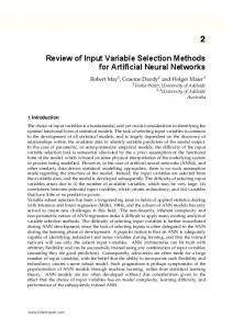
When performing variable selection for clustering, the goal is to retain only the relevant variables. With this aim, is crucial to define what it means for a variable to be, or not to be, “relevant”. In supervised learning the matter has been object of rigorous discussion for long time; we mention the works of Yu and Liu (2004), Blum and Langley (1997), Kohavi and John (1997), Koller and Sahami (1996) and John et al. (1994). Within the model-based clustering approach, the question has been addressed recently in Ritter (2014). Model-based clustering places the clustering task into a formal modeling framework and the group structure is embedded in the group membership variable (McLachlan and Basford, 1988). In this case, the definition of relevance can be expressed in terms of probabilistic dependence (or independence) statements with respect to this variable (Ritter, 2014). Relevant variables contain the essential clustering information. In a model-based clustering context, their distribution directly depends on the group membership variable. On the other hand, irrelevant variables do not convey any beneficial information. These can be further divided into redundant and uninformative variables. Redundant variables provide information of similar quality to that already available in the relevant ones, therefore are not needed for a parsimonious modeling. In many situations, they contain similar information because they are correlated to the relevant ones. In terms of distributional representation, we may think of redundant variables as conditionally independent of the grouping variable given the relevant variables. They could be useful for clustering, but only if the relevant ones are not present. On the contrary, uninformative variables possess no discriminative information whatsoever. They correspond to noise and their distribution is completely independent of the group structure. Different model-based clustering and variable selection strategies can be delineated by distributional assumptions on relevant and irrelevant variables. Two main assumptions are peculiar to the task of variable selection and mixture model clustering; these are: • Local independence assumption. The relevant variables are conditionally independent within the groups. • Global independence assumption. The irrelevant variables are independent of relevant clustering variables. Figure 1 gives a simple sketch of the two independence statements. In specifying a general strategy for model-based clustering and selection of variables, these assumptions can be combined 2

z

X1

X2

z

X3

X1 X2 X3

(a) Local independence assumption

X4 X5

(b) Global independence assumption

Figure 1: Local and global independence assumptions. In the example, z is the group membership variable, X1 , X2 and X3 are relevant clustering variables, while X4 and X5 are irrelevant and not related to z. Under the local independence assumption there are no edges among the relevant variables. Under the global independence assumption there is no edge between the set of relevant variables and the set of irrelevant ones.

together or employed separately. They have different implications on the clustering model and the model for the relations among the variables. In particular, the local independence assumption helps to simplify the modeling of the joint distribution of relevant variables and is especially useful in high-dimensional data settings. It is a standard assumption of the latent class analysis model (Clogg, 1988). For Gaussian mixture models, the statement corresponds to assume components with diagonal covariance matrices. The global independence assumption implies that the joint distribution of the variables factors into the product of the mixture distribution of the relevant variables and the distribution of the irrelevant variables. The term “global” is used because the independence statement affects the distribution of all the variables, not only the clustering ones. This assumption simplifies the modeling of the relation between relevant and irrelevant variables. However, it limits the capability of taking into account the presence of redundant variables (Law et al., 2004, Raftery and Dean, 2006). Many of the methods that are presented in this review make use of one of the two assumptions above, either implicitly or explicitly. Likewise, how the variable selection algorithm interacts with the model fitting process defines the overall approach to the problem. For a general learning task, the principal distinction is in whether the selection is carried out separately or jointly to the learning procedure (John et al., 1994, Dash and Liu, 1997, Dy and Brodley, 2004, Saeys et al., 2007, Liu and Motoda, 2007). The first case corresponds to filter methods, where the selection is performed as a pre (or sometimes post) processing step. The second corresponds to wrapper methods, that combine learning and variable selection at the same time. In this case the selection procedure is “wrapped” around the learning algorithm. Filter approaches are easy to implement and computationally efficient. However, wrapper methods often provide superior results, despite being more involved (Blum and Langley, 1997, Kohavi and John, 1997, Guyon and Elisseeff, 2003). In model-based clustering, filter methods perform the variable selection before (or after) the model has been estimated. The inferred classification is then used to evaluate the quality of the variables. In contrast, with a wrapper method model estimation and selection are conducted simultaneously. Variables selected via filter methods can miss important information as the selection is external to the model estimation. Indeed, wrapper methods have recently attracted most of the attention and are the most widespread. Their advantages lie in the fact that they can be naturally included in the model fitting, can lead to a better classification and can provide a better representation of the data generating process (Dy and Brodley, 2004, Law et al., 2004). 3

Within the class of wrappers, the various methods for variable selection in mixture model clustering can be further distinguished according to the type of statistical approach used. Three major approaches can be found in the literature: • Bayesian approaches. In this class of methods, the problem of variable selection is addressed assuming the existence of a latent variable indicating if an observed variable characterizes a mixture distribution or not. Variable selection is conducted by making inference about the posterior distribution of such a latent variable. • Penalization approaches. Within this category, variable selection is performed by using a penalized log-likelihood approach. The penalization term is a function of the mixture parameters and acts to shrink the estimates towards an overall common value. Variables whose estimates take this common value across the different mixture components are considered irrelevant and are discarded. • Model selection approaches. Here the task of variable selection is re-formulated as a model selection problem. Different models are specified according to the role of the variables towards the clustering structure. Consequently, relevant variables are selected by comparing different models using some predefined criterion. The above categorization is not exhaustive nor are the definitions intended to be mutually exclusive. Indeed, many of the methods that will be presented in the rest of the paper have some degree of overlap and a method belonging to one type of approach could be easily rephrased in terms of the other ones. These three general approaches are the predominant in the literature and the classification will be used for ease of exposition and a systematic presentation. In summary, the existing variable selection methods for model-based clustering are differentiated in relation to the distributional assumptions for relevant and irrelevant variables, the interaction between variable selection and model fitting, and the general statistical approach. We will give an overview of these methods after a short description of the model-based clustering framework.

3

Model-based clustering

Let X be the N ×J data matrix, where each row xi = (xi1 , . . . , xij , . . . , xiJ ) is the realization of a J-dimensional vector of random variables X = (X1 , . . . , Xj , . . . , XJ ). Model-based clustering assumes that each observation arises from a finite mixture of G probability distributions, each representing a different cluster or group (Fraley and Raftery, 2002, Melnykov and Maitra, 2010, McNicholas, 2016). The general form of a finite mixture distribution is specified as follows: p(xi ; Θ) =

G X

τg p(xi ; Θg ),

(1)

g=1

where the τg are the mixing probabilities and Θg is the parameter set corresponding to component g; Θ denotes the set of all parameters of the mixture. The component densities fully characterize the group structure of the data and each observation belongs to the corresponding cluster according to a latent cluster membership indicator variable zi = (zi1 , . . . , zig , . . . , ziG ), such that zig = 1 if xi arises from the gth subpopulation (McLachlan and Peel, 2000, McLachlan and Basford, 1988). For a fixed number of components, parameters are usually estimated using the EM algorithm (Dempster et al., 1977, McLachlan and Krishnan, 2008, Bartholomew et al., 2011, O’Hagan 4

et al., 2012). Moreover, generally model selection corresponds to the selection of the number of components G and to accomplish the task a plethora of methods have been suggested in the literature, the Bayesian Information Criterion (BIC, Schwarz, 1978) being the most popular one. Another popular approach for mixture model selection is the Integrated Complete-data Likelihood criterion (ICL, Biernacki et al., 2000), which gives more importance to model with well separated clusters. See McLachlan and Rathnayake (2014) for a detailed review of the various methods. After parameters have been estimated, each observation is assigned to the corresponding cluster using the maximum a posteriori (MAP) rule (McLachlan and Peel, 2000, McNicholas, 2016). The posterior probabilities uig = Pr(zig = 1 | xi ) of observing cluster g given the data point i are estimated as follows: ˆ g) τˆg p(xi ; Θ , uˆig = PG ˆ τ ˆ p(x ; Θ ) h i h h=1 Then observation xi is assigned to cluster g if g = MAP(ˆ ui ) = argmax {ˆ ui1 , . . . , uˆih , . . . , uˆiG }. h

According to the nature of the data, different specifications for the component densities in (1) have been proposed. In the following sections we focus on the cases of continuous and categorical data, taking in consideration the two most popular distributions: Gaussian and Multinomial. However, various and more flexible distributional assumptions can be specified, enabling to take into account for skewness, heavy tails and different data types; for example, see McNicholas (2016) for a review on non-Gaussian components, Karlis and Meligkotsidou (2007) for clustering multivariate count data, McParland and Gormley (2016) for mixed data modelbased clustering, Kosmidis and Karlis (2016) for the use of copulas in model-based clustering, DeSantis et al. (2008) for latent class analysis of ordinal data.

3.1

Gaussian mixture model

When clustering multivariate continuous data, a common approach is to model each component density by a multivariate Gaussian distribution. For a Gaussian mixture model (GMM) the mixture density in (1) becomes: p(xi ; Θ) =

G X

τg φ(xi ; µg , Σg ),

(2)

g=1

where φ is the multivariate Gaussian density and µg and Σg are the mean and covariance parameters respectively; see Fraley and Raftery (2002), Melnykov and Maitra (2010) and McNicholas (2016) for reviews. To attain parsimony, several approaches involving re-parameterizations of the covariance matrix Σg have been presented; for example Banfield and Raftery (1993), Celeux and Govaert (1995), Bouveyron et al. (2007), McNicholas and Murphy (2008), Biernacki and Lourme (2014). We refer to Bouveyron and Brunet-Saumard (2014b) for a review. Model based-clustering via GMMs can be performed in R (R Core Team, 2017) using the packages mclust (Scrucca et al., 2016), Rmixmod (Lebret et al., 2015) and flexmix (Leisch, 2004).

5

3.2

Latent class analysis model

For clustering multivariate categorical data, the common approach is to use the latent class analysis model (LCA, Bartholomew et al., 2011). Under this model, the mixture density in (1) is a mixture of Multinomial distributions as follows: p(xi ; Θ) =

G X g=1

where C(xi ; πg ) =

τg C(xi ; πg ),

Cj J Y Y 1{xij =c}

πgjc

(3)

,

j=1 c=1

with πgjc representing the probability of occurrence of category c for variable Xj in class g and Cj the number of categories of variable j. The factorization in C(xi ; πg ) is due to the local independence assumption, stating that the variables are independent within each latent class (Clogg, 1988). More details about the model can be found in Vermunt and Magdison (2002), Agresti (2002), Collins and Lanza (2010). For different values of G, not all the models can be fitted and constrains on the parameters need to be placed in order to ensure identifiability (Goodman, 1974); for examples see Formann (1985). R packages implementing the LCA model for clustering categorical data are BayesLCA (White and Murphy, 2014), poLCA (Linzer and Lewis, 2011) and flexmix (Leisch, 2004).

4

Variable selection methods for Gaussian mixture models

In this section we provide an overview of the available methods for clustering and variable selection using Gaussian mixture models. Steinley and Brusco (2008) and Celeux et al. (2014) compare and evaluate the performances of some of the methods described in the subsequent sections.

4.1

Bayesian approaches

Various methods have been developed within the Bayesian paradigm for simultaneous modelbased clustering and variable selection. A common feature among them is the introduction of a variable ϕ, usually following a distribution p(ϕ). The variable splits X into two sets: XC , the set of variables defining a Gaussian mixture distribution, and XN C , the set of variables indicating a single multivariate Gaussian distribution. In its most general form, the distribution of the data, conditional on z, can be expressed as: p(X | z, G, ϕ, Ω) = p(XC | z, G, ϕ, Θ) p(XN C | ϕ, Γ), with p(XC | z, G, ϕ, Θ) a mixture distribution whose parameters are denoted by Θ, p(XN C | ϕ, Γ) a single Gaussian distribution with parameters Γ, and Ω denoting the collection {Θ, Γ} of all parameters. Then, with the aim of variable selection and clustering, the focus is in drawing inference from the posterior distribution: p(z, G, ϕ, Ω | X) ∝ p(X | z, G, ϕ, Ω) p(z | Ω) p(G) p(ϕ) p(Ω). 6

In this context, Liu et al. (2003) propose the anchor mode model, where variable selection is performed by selecting the most informative principal components (or factors) of the data. In this approach, a preliminary dimension reduction through principal component analysis is performed and the first k0 factors are retained. Then it is assumed that only a subset of these factors is informative for clustering and distributed according to a mixture of Gaussians, while the remaining components follow a simple Gaussian distribution. The subset consists of the first ϕ principal components, where ϕ is a random variable distributed according to the prior distribution p(ϕ). Inference on this number of relevant factors is conducted employing a Markov Chain Monte-Carlo (MCMC) scheme where the prior p(ϕ) is taken to be the Uniform distribution, and the method is shown to perform well on high-dimensional gene expression data. However, selection is performed on a set of features derived from the original variables and in general the principal components with the larger eigenvalues will not necessarily contain the most information about the clustering (Chang, 1983). As an alternative to the “hard selection” approach (a variable is either selected or not), Law et al. (2004) suggest a Bayesian framework where the concept of feature saliency is introduced. Let ϕ = (ϕ1 , . . . , ϕj , . . . , ϕJ ) be a binary variable such that ϕj = 1 if Xj is relevant and ϕj = 0 otherwise. Then the saliency of variable Xj is the quantity ρj = Pr(ϕj = 1) and can be interpreted as the importance of the variable in characterizing the cluster structure of the data. Assuming conditional independence of the variables, it follows that the likelihood of a data-point can be expressed as: p(xi | Ω) =

G X g=1

τg

J h Y j=1

i

ρj φ(xij | µg , σg2 ) + (1 − ρj ) φ(xij | Γ) ,

with clear use of the notation. Rather than ϕ, the interest here is in recovering the probabilities ρj and a Dirichlet prior is placed on the corresponding vector. To encourage the saliences of some variables to converge to zero, the authors adopt a minimum message length criterion (Wallace and Freeman, 1987) and utilize an EM algorithm for maximum a posteriori estimation. Within the same framework, Constantinopoulos et al. (2006) consider a variational learning method for estimating the saliences. The same idea of a binary clustering-relevance indicator variable ϕ is employed in Tadesse et al. (2005). The authors assume a prior on ϕ of the form: p(ϕ | η) =

J Y j=1

η ϕj (1 − η)1−ϕj ,

with η the hyper-parameter interpreted as the proportion of variables expected to discriminate the groups. A MCMC scheme is used for inference, and the vector ϕ is updated using a Metropolis search where a new candidate is generated from previous state by adding, removing and swapping at random their entries. Posterior inference on ϕ is drawn after integrating out the parameters and considering the marginal posterior p(ϕj = 1 | X). Then the best clustering variables can be identified as those with largest marginal posterior, p(ϕj = 1 | X) > t, with a specified t. Alternatively, the selection can be performed by taking into account the complete vector ϕ with largest posterior probability among all visited vectors throughout the chain, thus considering the joint density of ϕ. The method is shown to perform well in clustering highdimensional microarray data. Furthermore, in subsequent work, Kim et al. (2006) extend the approach by formulating the clustering in terms of an infinite mixture of Gaussian distributions via Dirichlet process mixtures, while Swartz et al. (2008) expand it to the modeling of data with a known structure imposed from an experimental design. 7

4.2

Penalization approaches

In this context, a penalization term is introduced on the model parameters and variable selection is performed by inducing sparsity in the estimates. The aim is in maximizing a penalized version of the log-likelihood under a Gaussian mixture model and discard those variables whose parameter estimates are shrunken to zero or to a common value across the mixture components. In its general form, this penalized log-likelihood is as follows: `Q =

N X

log

 G X 

i=1

g=1

 

τg φ(xi ; Θg ) − Qλ (Θ),

(4)



where the penalization term Qλ (Θ) is a function of the Gaussian densities parameters Θ and λ, a generic penalty parameter (here in the notation we denoted with Θ the collection of all Gaussian density parameters and with Θg the subset corresponding to component g). Generally, the various methods are differentiated by the form of the function Qλ (·), having different implications on the selection of variables. Seminal work in this class of approaches is the method introduced by Pan and Shen (2007). The authors use a L1 penalty function of the form: λ

G X J X g=1 j=1

| µgj | .

After centering the data, the method realizes variable selection by automatically shrinking several small estimates of µgj towards zero. Indeed, if µgj = 0 for all g, the component means for variable j are equal to the overall data mean and variable j does not contribute to the clustering. A closely related approach is the one suggested by Bhattacharya and McNicholas (2014), where the penalizing function accounts for the size of the clusters and is given by: G X

λ

J X

N τg

g=1

j=1

| µgj | .

The parameter λ depends on the sample size and the authors derive a BIC-type model selection criterion for high-dimensional settings. The L1 penalty function treats each µgj individually, not using the information that, across the mixture components, the parameters (µ1j , . . . , µgj , . . . , µGj ) corresponding to the same variable Xj are grouped. This results in the fact that, if for a fixed variable j and some component g, we have µgj 6= 0 while µkj = 0 for all the remaining components, then the variable would not be excluded. Wang and Zhu (2008) suggest a solution to the problem by replacing the L1 norm with the L∞ norm. Thus the penalty function is given by: λ

J X j=1

max { | µ1j | , . . . , | µgj | , . . . , | µGj | }. g

After re-parameterizing µgj = αj βgj (αj ≥ 0), the authors consider also a hierarchical penalization function of the form: λ1

J X

j=1

αj + λ2

G X J X

g=1 j=1

| βgj | ,

with λ1 controlling the amount of shrinkage on the µgj as a group for g = 1, . . . , G, and λ2 controlling the shrinkage effect within variable j. This function has the advantage of being more 8

flexible and inducing a less “hard” penalization than the L∞ norm. Both penalty functions take into account the fact that component means corresponding to the same variable can be treated as grouped and tend to conduct a more effective variable selection. The idea of grouped parameters is also accounted in Xie et al. (2008b). Here the authors suggest the use of two planes of grouping: vertical and horizontal mean grouping. For the first, mean parameters afferent to the same variable are treated as a whole and the penalty function is: J √ X || µj ||2 λ G j=1

where µj = (µ1j , . . . , µgj , . . . , µGj ) and ||·||2 denotes the L2 norm. The same idea is exploited in the horizontal grouping, where prior knowledge that some variables work in groups is introduced in the penalization. Here the variables can be grouped in M groups indexed by m and each one of size Hm . Then the function is given by: λ

G X M q X g=1 m=1

Hm || µgm ||2 ,

with µgm the vector of means of component g for variables in group m. The two planes of penalization can be combined together and Xie et al. (2008b) show their superior performance in comparison to the standard L1 penalty. An approach allowing to identify which variables are discriminative for which specific pairs of clusters is the one proposed by Guo et al. (2010). They introduce a pairwise fusion penalty of the form:   λ

G X X

J X

 j=1

g=1 h