Documento de Trabajo 2005-06 Facultad de Ciencias Económicas y Empresariales Universidad de Zaragoza
Model selection strategies in a spatial context. Jesús Mur (*) Ana Angulo (**) University of Zaragoza. Department of Economic Analysis Gran Vía, 2-4 (50005) Zaragoza, (SPAIN) Phone: +34-976-761815 (*)
[email protected] (**)
[email protected]
Abstract: This paper follows on from the discussion of Florax, Folmer and Rey (2003) on the advantages and disadvantages of various specification strategies for econometric models in a spatial setting. Habitual practise has popularised a technique based on the well-known Lagrange Multipliers, which seems to give good results although its basis is entirely ad hoc. In this paper we also contemplate other alternatives which, from a strictly theoretical point of view, seem to be more elaborated. We focus attention on the problem of deciding which model should be specified once the initial one, generally static, presents symptoms of misspecification. There are two alternatives habitually contemplated, the Spatial Lag Model and the Spatial Error Model, which leads us to a classical decision problem. In the final part of the paper we present the results of a Monte Carlo exercise which has enabled us to clear up some doubts, although others still persist. JEL Classification: C21 Keywords: Model selection; Spatial Econometrics; Cross-sectional dependence Acknowledgements: This work has been carried out with the financial support of project SEC 2002-02350 of the Ministerio de Ciencia y Tecnología del Reino de España.
DTECONZ 2005-06: J.Mur and A.Angulo
1- Introduction Generally speaking, it could be said that there are hundreds of different ways of dealing with the problem of specifying an econometric model. Obviously, it is unlikely that all of them would finish up with the same equation. Thus, the question of the method of selecting, and discarding, models arises as one of the most important for us when doing applied econometrics. In a recent paper, Florax, Folmer and Rey (2003, FFR from now on), review the strategies of specifying models in the area of Spatial Econometrics. According to them, at present, a classical forward stepwise approach dominates, structured in three steps: (i)- A simple model is specified, usually static, under ideal conditions. (ii)-A series of tests (of spatial dependence) are applied to the estimated equation. (iii)- If the null is rejected in any of the tests, some adjustments will be applied: reformulating the equation, filtering the variables, incorporating elements of spatial dynamics, etc. This method could be called Specific to General Modelling and is very popular among econometricians. Implicitly, the reliability of the procedure depends on the number and quality of the misspecification tests carried out during the process, which may explain the wide range of such tests habitually reported. As FFR indicate, we could adopt exactly the opposite approach in a ‘Hendry-like specification strategy’ structured in the following steps: (i)- Estimate the most ample model consistent with theory. (ii)-Test a series of simplifying assumptions until no more restrictions are accepted. (iii)- Test the overall robustness of the final specification using theoretical as well as statistical considerations. In case of doubts, return to (i). The paper of FFR focuses on comparing both approaches. They find that the first approach tends to perform better than the second. This is an interesting result, but the literature on econometric model selection is not limited to just these two broad approaches. There are other techniques that have proven useful in different situations. 1
DTECONZ 2005-06: J.Mur and A.Angulo
For example, the role of the Bayesian methodology cannot be ignored because it occupies a central position in the discussion. In applied econometrics, an approach based on the Kullback-Leiber information measure dominates. The AIC or the SBIC statistics are well-known criteria related to this measure and they are produced routinely. In this paper we will focus our attention on the proposals of Vuong (1989) and Clarke (2003). The first introduces another way of dealing with the Kullback-Leiber information measure, whereas the second produces a very simple criterion of model selection, rooted in the maximum likelihood estimation. The problem posed in both cases involves only two different Data Generating Processes (DGP). These models could be nested, overlapped or non-nested in the case of Vuong but must be non-nested in the analysis of Clarke. The restriction of having only two DGPs may appear too tight for both methods to be useful, although this situation is very common in applied spatial econometrics. This gives the Vuong and the Clarke test a role. In the second section we summarise a series of results, well established in mainstream econometrics, on the problem of how to compare models, paying special attention to the above-mentioned proposals of Vuong and Clarke. The third section describes the search strategies that dominate in a spatial context, as discussed in FFR. Next, in the fourth section of the paper, we will solve a brief simulation that may help us to compare the performance of the different approaches discussed previously. Section 5 presents some conclusions and prospects for future research.
2- Discriminating among econometric models. Some (well-known) keys. The question of how to discriminate between rival models has always had an important place in the research agenda of Econometrics. The decisions adopted in this respect will severely condition both the method of the research itself and the results derived from it. Nevertheless, practice continues to be very heterogeneous and, on many occasions, not very well-reasoned, which means that it is necessary to delve even deeper into the discussion. In spite of the surprising claim of Hausman (1992, p. 32) when he states that ‘the Economic method is deductive’, during recent decades there has been a strengthening of
2
DTECONZ 2005-06: J.Mur and A.Angulo
the consensus on the positivist tradition, in which the preferentialist approach predominates over the normative. As Popper (1979, p. 13) says: ‘The theoretician, I will assume, is essentially interested in truth, and especially in finding true theories. But when he has fully digested that we can never justify empirically -that is, by tests statements- the claim that a scientific theory is true, and that we are therefore at best always faced with the question of preferring, tentatively, some guesses to others, then he may consider from the point of view of a seeker for true theories, the question: What principles of preference should we adopt? Are some theories ‘better’ than others?’. This reasoning requires ‘falsifying’, systematically confronting the theories with the data and among themselves, which has contributed to consolidating a series of basic principles, such as the Information Criterion (Akaike, 1973) or that of Encompassment (Mizon, 1984). Furthermore, the consistency of the Bayesian approaches has generalised the use of concepts like Loss Function, Prior Distribution or Decision Criteria. We do not intend to follow this question any further as it clearly goes beyond the modest objectives of this paper (for a review of the state of the question, see, for example, Morgan, 1990, Ripley, 1996, or Burnham and Anderson, 2002). We only wish to highlight certain questions relevant to our case. In general terms, two broad strategies to resolve the problem of model discrimination can be identified. Dastoor and McAleer (1989) refer to them as Model Selection strategy, with which we look for the best model among various alternatives, and Hypotheses Testing strategy, where we test whether one model in particular is admissible. The difference between them, as is demonstrated in Aznar (1989), depends on the loss function assumed by the researcher. In normal circumstances (unless there are very well-defined preferences a priori in favour of one specification) the first strategy seems preferable, although in habitual practice the second type dominates. The approach that FFR call ‘‘classical’ specification search’ in spatial econometrics belongs to the latter category: it involves a succession of nested models using a stepwise forward method. The problems arise when we try to use the same approach with a collection of non-nested models because, as Chow (1983) indicates, the adequate tests are not the same and the interpretation of the results also differs. In this case, four different techniques can be identified to deal with the problem of discrimination between nonnested models (Clarke, 2004). The best-known are the Bayesian approaches and the
3
DTECONZ 2005-06: J.Mur and A.Angulo
traditional model selection criteria. The others are the test of Cox (1961), and its derivations in the J and JA tests of Davidson and MacKinnon (1981) and Fisher and McAleer (1979), respectively, together with model selection tests, particularly those of Vuong (1989) and the Distribution-Free test of Clarke (2003). The test of Cox is complex, especially when the equations are non-linear, and confusing in many cases because, as a result of the logic of the test, it allows both models to be accepted or rejected simultaneously. However, its use has become popular through the J and JA tests. The Bayesian reasoning is very attractive, though it is also not exempt from criticism. The posterior odds combine the prior odds with the Bayes factor, which measures the change in the priors due to the sampling information. The first problem is to define the prior odds (Lesage, 2004, proposes very interesting solutions). However, as Clarke (2004, p.3) indicates: ‘(...) the Bayes factor does not provide a measure of support for one model over another, but rather it measures “the change in the odds in favor of the hypothesis when going from prior to the posterior”1’. The most extended technique to compare models in a context of non-nested models uses one, or various, of the wide range of model selection criteria available in the literature. Possibly the most popular is the AIC of Akaike (1973), or its Bayesian version, the SBIC (Schwarz, 1978), included systematically in almost all the software applications. The main advantage of this line lies in its simplicity and the clarity of its results. The selection criterion used will always choose the best model according to the internal philosophy of the criterion. Nevertheless, in many situations the differences between the models are hardly appreciable and will not be reflected in the working of the selection criterion. The novelty that the model selection tests bring with respect to the criteria is that they explicitly contemplate a situation of indifference between the alternatives to choose from. If the available evidence is not sufficiently clear in favour of one of the models, it is important to transmit this information to the user so that he can decide accordingly. The main difference lies in the firmer exploitation of the statistical elements associated with the problem of the decision to be carried out in the second option. The final results are not, necessarily, more complex. Otherwise, the essential reasoning underlying the approaches of the criteria and of the tests of selection are basically the same. 1
In the original, quoted from Lavine and Schervish (1999).
4
DTECONZ 2005-06: J.Mur and A.Angulo
The test of Voung (1989) can be presented as a reinterpretation of the test of Cox (1961). In the latter we have two families of conditioned density functions:
f θ = {f Y|X (θ); θ ∈ Θ ⊂ ℜ
}
p
{
}
and g γ = g Y|X ( γ ); γ ∈ Γ ⊂ ℜ q , and we want to test one
against the other. The null hypothesis corresponds to one of the families while the other is the alternative ( H 0 : f θ vs. H A : g γ ). The Cox statistic is a centred and typified version of the traditional Likelihood Ratio: C 0(f ) =
LR n (θ% n; γ% n ) − E Z E f ( LR n (θ% n; γ% n ) ) V ⎡⎣ LR n (θ% n; γ% n ) − E Z E f ( LR n (θ% n; γ% n ) ) ⎤⎦
~ N ( 0,1) as
(2.1)
Where θ% n and γ% n are the respective ML estimations of θ and γ and LRn is the Likelihood Ratio ( LR n (θ% n; γ% n ) = L f (θ% n ) − L g ( γ% n ) ). Next, the test should be repeated taking the other density function g γ in the null hypothesis. The problem with this reasoning is that the model of the alternative hypothesis only has power to accept or reject the model of the null hypothesis, which is a potential source of conflict. Vuong (1989) uses the structure of inference of the test of Cox, but redefines the content of the null and alternative hypotheses. Now, the former is associated with a situation of indifference between the models (taking into account the sample evidence), while the alternative is bilateral and identifies the model most favoured by the data. In analytical terms: ⎫ ⎪ ⎪ ⎪ ⎧ f (Y t | X t; θ) ⎤ ⎪ 0⎡ > 0⎬ ⎪ H f : E ⎢lg ⎥ ⎪ ⎣ g(Y t | X t; γ ) ⎦ ⎪ HA : ⎨ ⎪ ⎪ : 0 ⎡lg f (Y t | X t; θ) ⎤ < 0 ⎪ ⎪H g E ⎢⎣ g(Y t | X t; γ ) ⎥⎦ ⎪⎭ ⎩ f (Y t | X t; θ) ⎤ 0⎡ H 0 : E ⎢ lg ⎥=0 ⎣ g(Y t | X t; γ ) ⎦
(2.2)
This change of perspective allows us to obtain additional results of convergence in probability and in distribution with respect to the LRn statistic of (2.1). The most important are summarised in the following expression:
5
DTECONZ 2005-06: J.Mur and A.Angulo
⎧⎪ LR n (θ% n; γ% n ) ⎡ f ( Y t | X t; θ ) ⎤ ⎫⎪ D 2 − E 0 ⎢ lg n⎨ ⎥ ⎬ → N(0; ω ) n ⎣ g ( Y t | X t; γ ) ⎦ ⎭⎪ ⎩⎪
⎫ ⎪ ⎪⎪ ⎬ ⎡⎛ f ( Y | X ; θ ) ⎞ 2 ⎤ ⎛ ⎡ f ( Y | X ; θ ) ⎤ ⎞ 2 ⎪ ⎡ ⎤ θ f | ; ( ) Y X t t t t t t 2 0 0 ω = V ⎢lg ⎟⎟ ⎥ − ⎜⎜ E 0 ⎢ lg ⎥ = E ⎢⎜⎜ lg ⎥⎟ ⎪ γ γ g | ; g | ; ⎢ ⎥ ⎝ ⎣ g ( Y t | X t; γ ) ⎦ ⎟⎠ ⎪ ( ) ( ) Yt Xt ⎦ Y X t t ⎣ ⎝ ⎠ ⎣ ⎦ ⎭
(2.3)
Finally, Theorem 5.1 of Vuong (1989, p. 318) establishes that: ‘.... if Fθ and Gγ are strictly non-nested, then: (i) under H 0 : n
−1 / 2
[
D
]
~ ~ ~ → N (0;1) LR n θ n ; γ n / ω n
[
as
]
~ ~ (ii) under H f : n−1 / 2 LR n ~ θ n ; γ n / ωn →+ ∞
[
]
as
~ ~ (iii) under H g : n−1 / 2 LR n ~ θ n ; γ n / ωn →− ∞ (...)’ Given that the two models are different, the acceptance of the null should be interpreted as meaning that the available evidence does not permit us to discriminate between both alternatives. With slight variations, the test can also be used in the case where the models are nested or overlapped. The Distribution-Free Test of Clarke is even more intuitive because it ‘(…) applies a modified paired sign test to the differences in the individual log-likelihoods from two nonnested models. Whereas the Vuong test determines whether or not the average log-likelihood ratio is statistically different from zero, the proposed test determines whether or not the median log-likelihood ratio is statistically different from zero. If the models are equally close to the true specification, half the individual loglikelihood ratios should be greater than zero and half should be less than zero’ (Clarke,
2004, p.6). In other words, the reasoning reproduces the discussion of Vuong, just substituting the average with the median. In this way:
6
DTECONZ 2005-06: J.Mur and A.Angulo
⎡ f (Y t X t; θ) ⎤ ⎡ f (Y t X t; θ) ⎤ > 0 ⎥ = 0.5 H 0 : Median ⎢lg ⎥ = 0 ⇒ H 0 : Pr ⎢lg ⎣ g(Y t Z t; γ ) ⎦ ⎣ g(Y t X t; γ ) ⎦ ⎧ ⎡ f (Y t X t; θ) ⎤ ⎪H f : Median ⎢lg ⎥>0 g( ; ) γ Y X t t ⎪ ⎣ ⎦ HA : ⎨ ⎡ f (Y t X t; θ) ⎤ ⎪ : Median lg H g ⎢ ⎥LM-ERR then estimate the spatial lag model using MLLAG. If LM-LAGLM-LE we choose the SEM model and, if the inequality is in the opposite sense, the SLM. Lastly, the third case that we contemplate in the exercise is characterised by the true model not belonging to the catalogue of decision alternatives. The data have been generated with a mixed model like the following: y = ρ1Wy + xβ + u ⎫ ⎪ u = ρ 2Wu + ε ⎬ ε ~iid ( 0;σ 2I ) ⎪⎭
(4.3)
However, the decision options that are contemplated are limited to the SEM or to the SLM of (4.2), both false in this setting. Figures (4.1) to (4.4) summarise the results obtained in the first case (Testing
Approach). In Figures (4.1) and (4.2) the data have been generated using an SEM model with a high signal-to-noise ratio (that is, a high R2) in Figure (4.1) and a low one in the second. Figures (4.3) and (4.4) reproduce the results obtained when the data have been generated using an SLM. The data we present in each case indicate the number of times, in percentages, in which the corresponding decision method chooses one of the two models. Moreover, VU(SLM) means Vuong test as the method and SLM as selected model, CL indicates Clarke test and LM is reserved for the Robust Multipliers. We do not present, in order to make the reading of the figures easier, the percentages corresponding to the case of indetermination. Lastly, in the four figures we have also included the LR-COM test of common factors. The series denominated LRCF corresponds to the number of rejections of the hypothesis of common factors or, put another way, the percentage of decisions taken by this test in favour of the SLM model. 15
DTECONZ 2005-06: J.Mur and A.Angulo
Figures (4.5) to (4.8) have the same structure but are associated with the Criteria
Approach. The change of focus means that there are no longer situations of indetermination (the sum of the series VU(SEM) and VU(SLM), for example, is 1, while in the previous case the result of the sum was less than or equal to 1). In this collection of figures we have not included the LR test of common factors. Lastly, in Figures 4.9 to 4.17 we summarise the results corresponding to the third case, in which the data have been generated with the mixed model of (4.3) and high Signal-to-Noise Ratio. The figures we include are bi-dimensional. Horizontally we reproduce the range of ρ1 (the coefficient that accompanies the spatial lag of y in the main equation of 4.3) and vertically the range of ρ2 (the dependence coefficient of the error term in 4.3). Each figure reflects the number of times that each test selects the model identified in the heading. In Figures (4.9) to (4.14) the so-called Testing
Approach is developed, in which situations of indifference are relevant, while in the last three the Criteria Approach is used (consequently, there is no place for uncertainty).
4.2- Main results of interest It is not very encouraging to begin this conclusions section by saying that ‘there is still a
lot of work to do’ though, in our case, the comment seems inevitable. Some aspects of the difficulties involved in the discrimination between models in a spatial context seem clearer now, but there remain many questions which we have been unable to answer. Among the former we want to mention the following: * There is an evident sample size effect that conditions the behaviour of all the methods examined. Their reliability improves substantially when the size of the sample increases from 25 to 100 observations. The leap from 100 to 225 observations also introduces improvements, although less pronounced. * The intensity of the autocorrelation, residual or substantive, is an even more determining factor than the sample size. The behaviour of the different method is deficient when the symptoms of autocorrelation are weak, but improves as we approach the extremes of the range of values admissible for the parameter. * Relevant changes in the results are not appreciable with respect to the weight of the systematic and random part of the equation. That is, the Signal-to-Noise Ratio factor is secondary.
16
DTECONZ 2005-06: J.Mur and A.Angulo
* The methods of discrimination seem biased towards models that contain a strong autocorrelation structure. That is, when SEM models are simulated, the zones of no determination, or of erroneous selections are often very broad, but the margins are sharp when the data has been obtained from SLM models. Generally speaking, we can say that there is a certain predisposition to select SLM models more frequently than is necessary. * The Robust Multipliers are not reliable when used in a Testing Approach. At the extremes of the parameter interval considered, situations of indefinition, in which both tests are significant, tend to dominate. This is why the percentage of correct decisions corresponding to the Robust Multipliers in Figures 4.1 and 4.2 falls at the extremes of the interval. If the data come from an SLM, the anomalies occur in a zone of intermediate values in the positive branch of the interval of parameters. The dimensions of the ‘bubbles’ produced in this case increase with the sample size. The consequences are dramatic when using a sample of 225 observations. Moreover, the reliability of the Multipliers deteriorates at the extremes of the parameter interval. * The Clarke test suffers from a similar effect when the data come from an SLM, although the size of the bubble decreases with the sample size. * The Vuong test seems to work (relatively) better then the Clarke test in the
Testing Approach, which contradicts the results obtained by Clarke himself (Clarke 2004; see also Clarke and Signorino, 2004). In any case, the best option in this setting is the LR-COM. * The bubbles disappear when these techniques are used in a Criteria Approach. The evolution of the series in Figures 4.5 to 4.8 is more consistent, although proximity to the extremes of the interval has pernicious effects on the Robust Multipliers. In this case, the falls tend to decrease with the sample size as well as with the Signal-to-Noise Ratio: the criterion based on the multipliers works better for equations with a high explicative power. * The Clarke test, except in certain cases associated with the SEM model, seems generally worse than the other two alternatives. It could be considered the third option in order of preference. * The differences between the results of the Vuong test and those of the Robust Multipliers are small, although the former is more consistent in the range of parameter
17
DTECONZ 2005-06: J.Mur and A.Angulo
considered and, generally, outperforms the latter. The Vuong test should be taken as the best option in this case. * The bias of all the discrimination methods considered in favour of the SLM alternative is evident in Figures 4.9 to 4.17. The bias is accentuated in the case of the LR-COM test, as is evident in Figure 4.14. * Vuong's test and Clarke's test tend towards indefinition (correct decision in this case) when the sample size is reduced. As it increases, the zones of no determination are compressed towards the diagonals of the parametric space. Simultaneously, there is an increase in the number of times that the SEM model and, very especially, the SLM are selected. This last option is the dominant one with a sample size of 225. * The direction of the movements is less clear in the case of the Robust Multipliers. The preference for the SLM model also dominates, but the increase of the sample size does not compress the zones of indefinition. Both tests tend to be nonsignificant, as we expected, around point (0,0), while both tend to be significant in the interior regions of the four quadrants. * The preference for SLM structures is much clearer when the analysis is resolved with a Criteria Approach. In the three cases represented in Figures 4.15 to 4.17, the decisions taken in favour of this model clearly dominate, relegating the SEM option to a thin band concentrated around the value zero for the parameter that accompanies the spatial lag in the main equation of the model.
5- Conclusions
With this paper we want to vindicate the importance of a stage that has occupied a secondary position in the process of elaboration of econometric models with a spatial context. During recent years, many results on estimation and test methods in this setting have been published, though references to how to discriminate between rival models have been scarce. In our paper we contemplate a very particular problem: how to discriminate between an SLM and an SEM model, once there are clear signs of misspecification in the initial static equation. Day to day practice has ended up consolidating some methods that, seemingly, work reasonably well. In the exercise that we have resolved, the simple 18
DTECONZ 2005-06: J.Mur and A.Angulo
comparison of the values of the Robust Multipliers, as a guide to choosing the most appropriate model, has obtained good results. It is a simple proposal, cheap (in terms of calculations) and relatively reliable. However, it is not the only available option. In the paper we have examined other alternatives that adapt well to the problem proposed. We have concentrated, in particular, on the model selection tests and the results are not disappointing. When we resolve the analysis in a Testing Approach, the behaviour of the tests of Vuong and of Clarke is more consistent than that of the Robust Multipliers. Nevertheless, the preferable option in this case is the traditional Likelihood Ratio of Common Factors. In a Criteria Approach, the test of Vuong is perfectly competitive against the Robust Multipliers, accepting the cost, evidently, of a greater complexity of calculation. The simulation exercise, and the previous discussion, have allowed us to resolve some questions though there are still many doubts that require additional work. The nature of the ‘bubbles’ that arise in the power functions of the Robust Multipliers is one of them. After discarding the existence of coding errors, we have not found a satisfactory explanation either for their cause or for the fact that their dimension increases with the sample size. There are also many other topics that we have not explicitly contemplated: heterogeneity, outliers, non normality, etc. The use of estimators other than the ML, more and more frequent in this setting, introduces new unknowns. Another question that still seems interesting to us is the apparently low reliability of what FFR (2003) call the ‘Hendry-like specification strategy’. It seems necessary to take up all of these aspects again at some time in the future.
19
DTECONZ 2005-06: J.Mur and A.Angulo
References
Akaike, H., 1973. Information theory and an extension of the maximum likelihood principle. In Petrov, B. and F. Cáski (eds.) Second International Symposium on Information Theory, pp. 267-281. Budapest: Akademiai Kaidó. Reprinted in Kort, S. and N. Johnson (eds): Breakthrougs in Statistics, volume I, pp. 599-624. Berlin: Springer. Anselin, L. and R. Florax, 1995. Small Sample Properties of Tests for Spatial Dependence in Regression Models: Some Further Results. In Anselin, L. and R. Florax (eds.) New Directions in Spatial Econometrics (pp. 21-74). Berlin: Springer. Anselin, L., A, Bera, R. Florax and M. Yoon, 1996. Simple Diagnostic Tests for Spatial Dependence. Regional Science and Urban Economics, 26, 77-104. Aznar, A., 1989. Econometric Model Selection: A New Approach. Dordrecht: Kluwer. Burnham, K. and D. Anderson, 2002. Model Selection and Multimodel Inference, 2nd edition. Berlin: Springer. Burridge, P., 1981. Testing for a common factor in a spatial autoregression model. Environment and Planning A, 13, 795-800. Charemza, W, and D. Deadman, 1997. New Directions in Econometric Practice. Cheltenham: Edward Elgar. Chow, A., 1983. Econometrics New York: McGraw-Hill. Clarke, K., 2003. Nonparametric Model Discrimination in International Relations. Journal of Conflict Resolutions, 47, 72-93. Clarke, K., 2004. A Simple Distribution-Free Test for Nonnested Hypothesis. Working Paper, Department of Political Science, University of Rochester. Clarke, K. and V. Signorino 2004. Discriminating Methods: Tests for Nonnested Discrete Choice Models. Working Paper, Department of Political Science, University of Rochester. Cox, D., 1961. Tests of Separate Families of Hypotheses Proceedings of the Fourth Berkeley Symposium on Mathematical Statiscis and Probability, 1, 105-123. Dastoor, N. and M. McAleer, 1989. Some New Comparisons of Joint and Paired Tests for Non-Nested Models under Local Hypotheses. Econometric Theory, 5, 83-94. Davidson, R. and J. MacKinnon, 1981. Several tests for model specification in the presence of alternative hypotheses Econometrica, 88, 781-793. Fisher, G. and M. MacAleer, 1979. On the interpretation of the Cox tests in Econometrics Economics Letters, 4, 145-150. Florax, R. and T. de Graaff, 2004. The Performance of Diagnostics Tests for Spatial Dependence in Linear Regression Models: A Meta-Analysis of Simulation Studies. In Anselin, L., R. Florax and S. Rey (eds.): Advances in Spatial Econometrics: Methodology, Tools and Applications, pp. 29-65. Berlin: Springer.
20
DTECONZ 2005-06: J.Mur and A.Angulo
Florax, R., H. Folmer and S. Rey, 2003. Specification Searches in Spatial Econometrics: the Relevance of Hendry’s Methodology. Regional Science and Urban Economics, 33, 557-579. Hagget P. , 1965. Locational analysis in human geography. Edward Arnold: London Hausman, D., 1992. The Inexact and Separate Science of Economics. Cambridge: Cambridge University Press. Hepple, L., 1995a. Bayesian Techniques in Spatial and Network Econometrics: 1. Model Comparison and Posterior Odds. Environment and Planning A, 27, 447469. Hepple, L., 1995b. Bayesian Techniques in Spatial and Network Econometrics: 2. Computational Methods and Algoritms. Environment and Planning A, 27, 615644. Lavine, M. and M. Schervish, 1999. Bayes Factors: What They Are and What They Are Not . The American Statistician, 53, 119-122. Lesage, J., 2004. Lecture 6: Model Comparison. Working Paper, Department of Economics, University of Toledo. Mizon, G., 1984. The Encompassing Approach in Econometrics. In Hendry, D. and K. Wallis (eds.) Econometrics and Quantitative Economics pp. 135-172. Oxford: Basil Blackwell. Morgan, M., 1990. The History of Econometric Ideas. Cambridge: Cambridge University Press. Popper, K., 1979. Objective Knowledge. An Evolutionary Approach. Oxford: Oxford University Press. Ripley, B., 1996. Pattern Recognition and Neuronal Networks. Cambridge: Cambridge University Press. Rivers, D. amd Q. Vuong, 2002. Model Selection Tests for Nonlinear Dynamic Models. The Econometrics Journal, 5, 1-39. Schwarz, C., 1978. Estimating the Dimension of a Model. Annals of Statistics, 6, 461464. Vuong, Q., 1989. Likelihood Ratio-Tests for Model Selection and Non-Nested Hypotheses. Econometrica, 57, 307-333.
21
DTECONZ 2005-06: J.Mur and A.Angulo
Appendix A: Misspecification tests used in the analysis. The tests described here always refer to a static model, such as: y = X
+ u.
This model has been estimated by LS, where σˆ 2 and βˆ correspond to the LS estimations and uˆ to the residual series. These tests are the following (see Florax and de Graaff, 2004, for the details): 2
LM-ERR Test:
⎛ uˆ ' Wuˆ ⎞ 1 LM − ERR = ⎜ ; T1 = tr [ W ' W + WW ] ⎟ ⎝ σˆ 2 ⎠ T1
LM-EL Test:
⎛ uˆ ' Wuˆ T uˆ ' Wy ⎞⎟ ⎜ − 1 ⎜ σˆ 2 R Jˆ ρ-β σˆ 2 ⎟⎠ LM − EL = ⎝ T12 − T1 R Jˆ ρ-β
LM-LAG Test:
1 ⎛ uˆ ' Wy ⎞ LM − LAG = ⎜ ⎟ R Jˆ ρ−β ⎝ σˆ 2 ⎠
LM-LE Test:
⎛ uˆ ' Wy uˆ ' Wuˆ ⎞ − ⎜ ⎟ σˆ 2 σˆ 2 ⎠ ⎝ LM − LE = R Jˆ ρ-β − T1
(A.1)
2
(A.2)
2
(A.3)
2
(A.4)
ˆ ˆ / σˆ 2 and M=[I-X(X’X)-1X’]. The four Moreover, R Jˆ ρ−β = T1 + (β'X'WMWXβ)
Lagrange Multipliers have an asymptotic χ2 ( 1 ) distribution.
22
DTECONZ 2005-06: J.Mur and A.Angulo
Appendix B: The Hybrid and the Classical strategy of FFR (2003) These strategies differ in the way that they solve situations of uncertainty, where the LM-ERR and the LM-LAG are statistically significant. In the so-called ‘classical
strategy’, we compare the value of both statistics in order to specify the model associated with the more significant: the SEM if LM-ERR>LM-LAG and the SLM if LM-ERR LM-LAG ⇔ LM-EL > LM-LE. The proof is simple although a bit tedious. Using the expressions of Appendix A:
LM-EL>LM-LE ⇒
⎛ uˆ ' Wuˆ T uˆ ' Wy ⎞⎟ ⎜ − 1 ⎜ σˆ 2 R Jˆ ρ-β σˆ 2 ⎟⎠ ⎝
2
⎛ uˆ ' Wy uˆ ' Wuˆ ⎞ − ⎜ ⎟ ˆ2 ˆ2 ⎠ σ σ ⎝ > R Jˆ ρ-β − T1
T12 T1 − R Jˆ ρ-β
2
(B.1)
Simplifying common terms, (B.1) reads as: 2
⎞ R Jˆ ρ-β ⎛ 2 ⎜ uˆ ' Wuˆ − T1 uˆ ' Wy ⎟ > ( uˆ ' Wy − uˆ ' Wuˆ ) ⇒ ⎜ ⎟ R Jˆ ρ-β T1 ⎝ ⎠
(B.2)
After solving for the squares and grouping terms, we obtain: ⇒
R Jˆ ρ-β T1
( uˆ ' Wuˆ ) 2 > ( uˆ ' Wy ) 2
(B.3)
That is: 2
1 ⎛ uˆ ' Wuˆ ⎞ 1 ⎛ uˆ ' Wy ⎞ > LM − EL > LM − LE ⇒ ⎜ ⎟ ⎜ ⎟ R Jˆ ρ-β ⎝ σˆ 2 ⎠ T1 ⎝ σˆ 2 ⎠
2
(B.4) LM − EL > LM − LE ⇔ LM − ERR > LM − LAG
23
DTECONZ 2005-06: J.Mur and A.Angulo
Figure 4.1: Testing Approach. DGP: SEM. High Signal-to-Noise Ratio. Figure 4.1A:. R=25. 1.0
0.9
0.8
0.7
0.6
0.5
0.4
0.3
0.2
0.1
-0.27
-0.24
-0.21
-0.18
-0.15
-0.12
-0.09
VU(SLM)
-0.06
-0.03
VU(SEM)
0.0 0.00
0.03
CL(SLM)
0.06
0.09
CL(SEM)
0.12
LRCF
0.15
0.18
LM(SLM)
0.21
0.24
0.27
LM(SEM)
Figure 4.1B:. R=100. 1.0
0.9
0.8
0.7
0.6
0.5
0.4
0.3
0.2
0.1
-0.25
-0.22
-0.19
-0.16
-0.13
-0.10
VU(SLM)
-0.07
0.0 -0.01
-0.04
VU(SEM)
0.02
CL(SLM)
0.05
0.08
CL(SEM)
0.11
0.14
LRCF
0.17 LM(SLM)
0.20
0.23
LM(SEM)
Figure 4.1C:. R=225. 1.0
0.9
0.8
0.7
0.6
0.5
0.4
0.3
0.2
0.1
-0.23
-0.20
-0.17
-0.14 VU(SLM)
-0.11
-0.08
VU(SEM)
-0.05
0.0 -0.02
CL(SLM)
0.01 CL(SEM)
24
0.04
0.07 LRCF
0.10 LM(SLM)
0.13
0.16 LM(SEM)
0.19
0.22
DTECONZ 2005-06: J.Mur and A.Angulo
Figure 4.2: Testing Approach. DGP: SEM. Low Signal-to-Noise Ratio. Figure 4.2A:. R=25. 1.0
0.9
0.8
0.7
0.6
0.5
0.4
0.3
0.2
0.1
-0.27
-0.24
-0.21
-0.18
-0.15
-0.12
-0.09
VU(SLM)
-0.06
0.0 0.00
-0.03
VU(SEM)
0.03
CL(SLM)
0.06
0.09
CL(SEM)
0.12
LRCF
0.15
0.18
0.21
LM(SLM)
0.24
0.27
LM(SEM)
Figure 4.2B:. R=100. 1.0
0.9
0.8
0.7
0.6
0.5
0.4
0.3
0.2
0.1
-0.25
-0.22
-0.19
-0.16
-0.13
VU(SLM)
-0.10
-0.07
0.0 -0.01
-0.04
VU(SEM)
0.02
CL(SLM)
0.05
CL(SEM)
0.08
0.11
LRCF
0.14 LM(SLM)
0.17
0.20
0.23
LM(SEM)
Figure 4.2C:. R=225. 1.0
0.9
0.8
0.7
0.6
0.5
0.4
0.3
0.2
0.1
-0.23
-0.20
-0.17
-0.14 VU(SLM)
-0.11
-0.08 VU(SEM)
-0.05
0.0 -0.02
0.01
CL(SLM)
0.04
CL(SEM)
25
0.07 LRCF
0.10
0.13
LM(SLM)
0.16
0.19
LM(SEM)
0.22
DTECONZ 2005-06: J.Mur and A.Angulo
Figure 4.3: Testing Approach. DGP: SLM. High Signal-to-Noise Ratio. Figure 4.3A:. R=25. 1.0
0.9
0.8
0.7
0.6
0.5
0.4
0.3
0.2
0.1
-0.27
-0.24
-0.21
-0.18
-0.15
-0.12
-0.09
VU(SLM)
-0.06
0.0 0.00
-0.03
VU(SEM)
0.03
CL(SLM)
0.06
0.09
CL(SEM)
0.12
LRCF
0.15
0.18
0.21
LM(SLM)
0.24
0.27
LM(SEM)
Figure 4.3B:. R=100. 1.0
0.9
0.8
0.7
0.6
0.5
0.4
0.3
0.2
0.1
-0.25
-0.22
-0.19
-0.16
-0.13
VU(SLM)
-0.10
-0.07
0.0 -0.01
-0.04
VU(SEM)
0.02
CL(SLM)
0.05
CL(SEM)
0.08
0.11
LRCF
0.14
LM(SLM)
0.17
0.20
0.23
LM(SEM)
Figure 4.3C:. R=225. 1.0
0.9
0.8
0.7
0.6
0.5
0.4
0.3
0.2
0.1
-0.23
-0.20
-0.17
-0.14 VU(SLM)
-0.11
-0.08 VU(SEM)
-0.05
0.0 -0.02
CL(SLM)
0.01 CL(SEM)
26
0.04
0.07 LRCF
0.10
0.13
LM(SLM)
0.16 LM(SEM)
0.19
0.22
DTECONZ 2005-06: J.Mur and A.Angulo
Figure 4.4: Testing Approach. DGP: SLM. Low Signal-to-Noise Ratio. Figure 4.4A:. R=25. 1.0
0.9
0.8
0.7
0.6
0.5
0.4
0.3
0.2
0.1
-0.27
-0.24
-0.21
-0.18
-0.15
-0.12
-0.09
VU(SLM)
-0.06
-0.03
VU(SEM)
0.0 0.00
0.03
CL(SLM)
0.06
0.09
CL(SEM)
0.12
LRCF
0.15
0.18
0.21
LM(SLM)
0.24
0.27
LM(SEM)
Figure 4.4B:. R=100. 1.0
0.9
0.8
0.7
0.6
0.5
0.4
0.3
0.2
0.1
-0.25
-0.22
-0.19
-0.16
-0.13
-0.10
VU(SLM)
-0.07
0.0 -0.01
-0.04
VU(SEM)
0.02
CL(SLM)
0.05
CL(SEM)
0.08
0.11
LRCF
0.14 LM(SLM)
0.17
0.20
0.23
LM(SEM)
Figure 4.4C:. R=225. 1.0
0.9
0.8
0.7
0.6
0.5
0.4
0.3
0.2
0.1
-0.23
-0.20
-0.17
-0.14 VU(SLM)
-0.11
-0.08
VU(SEM)
-0.05
0.0 -0.02
CL(SLM)
0.01 CL(SEM)
27
0.04
0.07 LRCF
0.10
0.13
LM(SLM)
0.16 LM(SEM)
0.19
0.22
DTECONZ 2005-06: J.Mur and A.Angulo
Figure 4.5: Criteria Approach. DGP: SEM. High Signal-to-Noise Ratio. Figure 4.5A:. R=25. 1.0
0.9
0.8
0.7
0.6
0.5
0.4
0.3
0.2
0.1
-0.27
-0.24
-0.21
-0.18
-0.15
-0.12
-0.09
-0.06
VU(SLM)
-0.03
0.0 0.00
VU(SEM)
0.03
0.06
CL(SLM)
0.09
0.12
CL(SEM)
0.15
0.18
LM(SLM)
0.21
0.24
0.27
LM(SEM)
Figure 4.5B:. R=100. 1.0
0.9
0.8
0.7
0.6
0.5
0.4
0.3
0.2
0.1
-0.25
-0.22
-0.19
-0.16
-0.13
VU(SLM)
-0.10
-0.07
-0.04
VU(SEM)
0.0 -0.01
0.02
CL(SLM)
0.05
CL(SEM)
0.08
0.11
LM(SLM)
0.14
0.17
0.20
0.23
LM(SEM)
Figure 4.5C:. R=225. 1.0
0.9
0.8
0.7
0.6
0.5
0.4
0.3
0.2
0.1
-0.23
-0.20
-0.17
-0.14
-0.11
VU(SLM)
-0.08
-0.05
VU(SEM)
0.0 -0.02
0.01
CL(SLM)
28
0.04 CL(SEM)
0.07
0.10 LM(SLM)
0.13
0.16
LM(SEM)
0.19
0.22
DTECONZ 2005-06: J.Mur and A.Angulo
Figure 4.6: Criteria Approach. DGP: SEM. Low Signal-to-Noise Ratio. Figure 4.6A:. R=25. 1.0
0.9
0.8
0.7
0.6
0.5
0.4
0.3
0.2
0.1
-0.27
-0.24
-0.21
-0.18
-0.15
-0.12
-0.09
-0.06
VU(SLM)
-0.03
0.0 0.00
VU(SEM)
0.03
0.06
CL(SLM)
0.09
0.12
CL(SEM)
0.15
0.18
LM(SLM)
0.21
0.24
0.27
LM(SEM)
Figure 4.6B:. R=100. 1.0
0.9
0.8
0.7
0.6
0.5
0.4
0.3
0.2
0.1
-0.25
-0.22
-0.19
-0.16
-0.13
-0.10
VU(SLM)
-0.07
0.0 -0.01
-0.04
VU(SEM)
0.02
CL(SLM)
0.05
0.08
CL(SEM)
0.11
0.14
LM(SLM)
0.17
0.20
0.23
LM(SEM)
Figure 4.6C:. R=225. 1.0
0.9
0.8
0.7
0.6
0.5
0.4
0.3
0.2
0.1
-0.23
-0.20
-0.17
-0.14 VU(SLM)
-0.11
-0.08
VU(SEM)
-0.05
0.0 -0.02
CL(SLM)
0.01 CL(SEM)
29
0.04
0.07 LM(SLM)
0.10
0.13 LM(SEM)
0.16
0.19
0.22
DTECONZ 2005-06: J.Mur and A.Angulo
Figure 4.7: Criteria Approach. DGP: SLM. High Signal-to-Noise Ratio. Figure 4.7A:. R=25. 1.0
0.9
0.8
0.7
0.6
0.5
0.4
0.3
0.2
0.1
-0.27
-0.24
-0.21
-0.18
-0.15
-0.12
-0.09
-0.06
VU(SLM)
-0.03
0.0 0.00
VU(SEM)
0.03
0.06
CL(SLM)
0.09
0.12
CL(SEM)
0.15
0.18
LM(SLM)
0.21
0.24
0.27
LM(SEM)
Figure 4.7B:. R=100. 1.0
0.9
0.8
0.7
0.6
0.5
0.4
0.3
0.2
0.1
-0.25
-0.22
-0.19
-0.16
-0.13 VU(SLM)
-0.10
-0.07
-0.04
VU(SEM)
0.0 -0.01
0.02
CL(SLM)
0.05
0.08
CL(SEM)
0.11
LM(SLM)
0.14
0.17
0.20
0.23
LM(SEM)
Figure 4.7C:. R=225. 1.0
0.9
0.8
0.7
0.6
0.5
0.4
0.3
0.2
0.1
-0.23
-0.20
-0.17
-0.14
-0.11
VU(SLM)
-0.08
-0.05
VU(SEM)
0.0 -0.02
0.01
CL(SLM)
30
0.04 CL(SEM)
0.07
0.10 LM(SLM)
0.13
0.16
LM(SEM)
0.19
0.22
DTECONZ 2005-06: J.Mur and A.Angulo
Figure 4.8: Criteria Approach. DGP: SLM. Low Signal-to-Noise Ratio. Figure 4.8A:. R=25. 1.0
0.9
0.8
0.7
0.6
0.5
0.4
0.3
0.2
0.1
-0.27
-0.24
-0.21
-0.18
-0.15
-0.12
-0.09
VU(SLM)
-0.06
-0.03
0.0 0.00
VU(SEM)
0.03
0.06
CL(SLM)
0.09
CL(SEM)
0.12
0.15
LM(SLM)
0.18
0.21
0.24
0.27
LM(SEM)
Figure 4.8B:. R=100. 1.0
0.9
0.8
0.7
0.6
0.5
0.4
0.3
0.2
0.1
-0.25
-0.22
-0.19
-0.16
-0.13
-0.10
-0.07
VU(SLM)
-0.04
VU(SEM)
0.0 -0.01
0.02
CL(SLM)
0.05
0.08
CL(SEM)
0.11
0.14
LM(SLM)
0.17
0.20
0.23
LM(SEM)
Figure 4.8C:. R=225. 1.0
0.9
0.8
0.7
0.6
0.5
0.4
0.3
0.2
0.1
-0.23
-0.20
-0.17
-0.14
-0.11
VU(SLM)
-0.08
-0.05
VU(SEM)
0.0 -0.02
0.01
CL(SLM)
31
0.04 CL(SEM)
0.07
0.10 LM(SLM)
0.13
0.16
LM(SEM)
0.19
0.22
DTECONZ 2005-06: J.Mur and A.Angulo
Figure 4.9: Testing Approach. DGP: Mixed. High Signal-to-Noise Ratio. Vuong and Clarke Test. Identification: SEM. Vuong test
Figure 4.9A: R=25.
Clarke test
Vuong test
Figure 4.9B: R=100.
Clarke test
Vuong test
Figure 4.9C: R=225.
Clarke test
32
DTECONZ 2005-06: J.Mur and A.Angulo
Figure 4.10: Testing Approach. DGP: Mixed. High Signal-to-Noise Ratio. Vuong and Clarke Test. Identification: SLM.. Vuong test
Figure 4.10A: R=25.
Clarke test
Vuong test
Figure 4.10B: R=100.
Clarke test
Vuong test
Figure 4.10C: R=225.
Clarke test
33
DTECONZ 2005-06: J.Mur and A.Angulo
Figure 4.11: Testing Approach. DGP: Mixed. High Signal-to-Noise Ratio. Vuong and Clarke Test. Identification: Indiference. Vuong test
Figure 4.11A: R=25.
Clarke test
Vuong test
Figure 4.11B: R=100.
Clarke test
Vuong test
Figure 4.11C: R=225.
Clarke test
34
DTECONZ 2005-06: J.Mur and A.Angulo
Figure 4.12: Testing Approach. DGP: Mixed. High Signal-to-Noise Ratio. Robust LM. Identification: Positive. Robust LM: SEM
Figure 4.12A: R=25.
Robust LM: SLM
Robust LM: SEM
Figure 4.12B: R=100.
Robust LM: SLM
Robust LM: SEM
Figure 4.12C: R=225.
Robust LM: SLM
35
DTECONZ 2005-06: J.Mur and A.Angulo
Figure 4.13: Testing Approach. DGP: Mixed. High Signal-to-Noise Ratio. Robust LM. Identification: Not Conclusive. Robust LM: NONE
Figure 4.13A: R=25.
Robust LM: BOTH
Robust LM: NONE
Figure 4.13B: R=100.
Robust LM: BOTH
Robust LM: NONE
Figure 4.13C: R=225.
Robust LM: BOTH
36
DTECONZ 2005-06: J.Mur and A.Angulo
Figure 4.14: Testing Approach. DGP: Mixed. High Signal-to-Noise Ratio. LR-COMMOM Factors. Identification: SEM. Figure 4.14A: R=25.
Figure 4.14B: R=100.
Figure 4.14C: R=225.
37
DTECONZ 2005-06: J.Mur and A.Angulo
Figure 4.15: Criteria Approach. DGP: Mixed. High Signal-to-Noise Ratio. Vuong test. Identification: SLM
Figure 4.15A: R=25.
Identification: SEM
Identification: SLM
Figure 4.15B: R=100.
Identification: SEM
Identification: SLM
Figure 4.15C: R=225.
Identification: SEM
38
DTECONZ 2005-06: J.Mur and A.Angulo
Figure 4.16: Criteria Approach. DGP: Mixed. High Signal-to-Noise Ratio. Clarke test. Identification: SLM
Figure 4.16A: R=25.
Identification: SEM
Identification: SLM
Figure 4.16B: R=100.
Identification: SEM
Identification: SLM
Figure 4.16C: R=225.
Identification: SEM
39
DTECONZ 2005-06: J.Mur and A.Angulo
Figure 4.17: Criteria Approach. DGP: Mixed. High Signal-to-Noise Ratio. Robust LM. Identification: SLM
Figure 4.17A: R=25.
Identification: SEM
Identification: SLM
Figure 4.17B: R=100.
Identification: SEM
Identification: SLM
Figure 4.17C: R=225.
Identification: SEM
40
DTECONZ 2005-06: J.Mur and A.Angulo
Documentos de Trabajo Facultad de Ciencias Económicas y Empresariales. Universidad de Zaragoza.
2002-01: “Evolution of Spanish Urban Structure During the Twentieth Century”. Luis Lanaspa, Fernando Pueyo y Fernando Sanz. Department of Economic Analysis, University of Zaragoza. 2002-02: “Una Nueva Perspectiva en la Medición del Capital Humano”. Gregorio Giménez y Blanca Simón. Departamento de Estructura, Historia Económica y Economía Pública, Universidad de Zaragoza. 2002-03: “A Practical Evaluation of Employee Productivity Using a Professional Data Base”. Raquel Ortega. Department of Business, University of Zaragoza. 2002-04: “La Información Financiera de las Entidades No Lucrativas: Una Perspectiva Internacional”. Isabel Brusca y Caridad Martí. Departamento de Contabilidad y Finanzas, Universidad de Zaragoza. 2003-01: “Las Opciones Reales y su Influencia en la Valoración de Empresas”. Manuel Espitia y Gema Pastor. Departamento de Economía y Dirección de Empresas, Universidad de Zaragoza. 2003-02: “The Valuation of Earnings Components by the Capital Markets. An International Comparison”. Susana Callao, Beatriz Cuellar, José Ignacio Jarne and José Antonio Laínez. Department of Accounting and Finance, University of Zaragoza. 2003-03: “Selection of the Informative Base in ARMA-GARCH Models”. Laura Muñoz, Pilar Olave and Manuel Salvador. Department of Statistics Methods, University of Zaragoza. 2003-04: “Structural Change and Productive Blocks in the Spanish Economy: An Imput-Output Analysis for 1980-1994”. Julio Sánchez Chóliz and Rosa Duarte. Department of Economic Analysis, University of Zaragoza. 2003-05: “Automatic Monitoring and Intervention in Linear Gaussian State-Space Models: A Bayesian Approach”. Manuel Salvador and Pilar Gargallo. Department of Statistics Methods, University of Zaragoza. 2003-06: “An Application of the Data Envelopment Analysis Methodology in the Performance Assessment of the Zaragoza University Departments”. Emilio Martín. Department of Accounting and Finance, University of Zaragoza. 2003-07: “Harmonisation at the European Union: a difficult but needed task”. Ana Yetano Sánchez. Department of Accounting and Finance, University of Zaragoza.
41
DTECONZ 2005-06: J.Mur and A.Angulo
2003-08: “The investment activity of spanish firms with tangible and intangible assets”. Manuel Espitia and Gema Pastor. Department of Business, University of Zaragoza. 2004-01: “Persistencia en la performance de los fondos de inversión españoles de renta variable nacional (1994-2002)”. Luis Ferruz y María S. Vargas. Departamento de Contabilidad y Finanzas, Universidad de Zaragoza. 2004-02: “Calidad institucional y factores político-culturales: un panorama inter.nacional por niveles de renta”. José Aixalá, Gema Fabro y Blanca Simón. Departamento de Estructura, Historia Económica y Economía Pública, Universidad de Zaragoza. 2004-03: “La utilización de las nuevas tecnologías en la contratación pública”. José Mª Gimeno Feliú. Departamento de Derecho Público, Universidad de Zaragoza. 2004-04: “Valoración económica y financiera de los trasvases previstos en el Plan Hidrológico Nacional español”. Pedro Arrojo Agudo. Departamento de Análisis Económico, Universidad de Zaragoza. Laura Sánchez Gallardo. Fundación Nueva Cultura del Agua. 2004-05: “Impacto de las tecnologías de la información en la productividad de las empresas españolas”. Carmen Galve Gorriz y Ana Gargallo Castel. Departamento de Economía y Dirección de Empresas. Universidad de Zaragoza. 2004-06: “National and International Income Dispersión and Aggregate Expenditures”. Carmen Fillat. Department of Applied Economics and Economic History, University of Zaragoza. Joseph Francois. Tinbergen Institute Rotterdam and Center for Economic Policy Resarch-CEPR. 2004-07: “Targeted Advertising with Vertically Differentiated Products”. Lola Esteban and José M. Hernández. Department of Economic Analysis. University of Zaragoza. 2004-08: “Returns to education and to experience within the EU: are there differences between wage earners and the self-employed?”. Inmaculada García Mainar. Department of Economic Analysis. University of Zaragoza. Víctor M. Montuenga Gómez. Department of Business. University of La Rioja 2005-01: “E-government and the transformation of public administrations in EU countries: Beyond NPM or just a second wave of reforms?”. Lourdes Torres, Vicente Pina and Sonia Royo. Department of Accounting and Finance.University of Zaragoza 2005-02: “Externalidades tecnológicas internacionales y productividad de la manufactura: un análisis sectorial”. Carmen López Pueyo, Jaime Sanau y Sara Barcenilla. Departamento de Economía Aplicada. Universidad de Zaragoza. 2005-03: “Detecting Determinism Using Recurrence Quantification Analysis: Three Test Procedures”. María Teresa Aparicio, Eduardo Fernández Pozo and Dulce Saura. Department of Economic Analysis. University of Zaragoza. 2005-04: “Evaluating Organizational Design Through Efficiency Values: An Application To The Spanish First Division Soccer Teams”. Manuel Espitia Escuer and Lucía Isabel García Cebrián. Department of Business. University of Zaragoza.
42
DTECONZ 2005-06: J.Mur and A.Angulo
2005-05: “From Locational Fundamentals to Increasing Returns: The Spatial Concentration of Population in Spain, 1787-2000”. María Isabel Ayuda. Department of Economic Analysis. University of Zaragoza. Fernando Collantes and Vicente Pinilla. Department of Applied Economics and Economic History. University of Zaragoza. 2005-06: “Model selection strategies in a spatial context”. Jesús Mur and Ana Angulo. Department of Economic Analysis. University of Zaragoza.
43