Modeling a Reconfigurable System for Computing the FFT in Place via Rewriting-Logic‡ Mauricio Ayala-Rincón1,*, Rodrigo B. Nogueira§,2,*, Carlos H. Llanos2,*, Ricardo P. Jacobi 3,*, Reiner W. Hartenstein4,+ 1 2 Departamentos de Matemática, Engenharia Mecânica, 3Ciência da Computação, *Universidade de Brasília, 4Fachbereich Informatik, +Universität Kaiserlautern
[email protected],
[email protected],
[email protected],
[email protected]
Abstract The growing adoption of reconfigurable architectures opens new implementation alternatives and creates new design challenges. In the case of dynamically reconfigurable architectures, the choice of an efficient architecture and reconfiguration scheme for a given application is a complex task. Tools for exploration of design alternatives at higher abstraction levels are needed. This paper describes the modeling and simulation of a dynamically reconfigurable hardware implementation of the Fast Fourier Transform – FFT using rewriting-logic. It is shown that rewriting-logic can be used as a framework for fast design space exploration, providing a quick evaluation of different reconfigurable solutions.
1. Introduction Reconfigurable Computing is a new research area which is gaining momentum due to the potential improvement that can be obtained when compared both to software solutions as well as to dedicated full-custom devices. When compared to software solutions running on general purpose processors, reconfigurable computing delivers more processing power due to the implementation of algorithms in hardware. A remarkable example in this case is DeCypher [9], a reconfigurable machine targeted to accelerate genetic related algorithms. It is built upon commercial FPGAs interconnected through a PCI bus and can improve the performance of genetic algorithms by some orders of magnitude. Several other examples can be drawn from telecommunication systems, in tasks such as data compression, encoding and decoding, and digital signal processing. On the other hand, reconfigurable computing provides more flexibility than dedicated full custom ASICs (Application Specific Integrated Circuits). ‡ §
Work supported by the CAPES-DFG Brazilian-German foundations. Author partially supported by the CNPq Brazilian council.
Moreover, the exploding costs of integrated circuits fabrics associated with shorter devices lifetimes makes the design of ASIC a very expensive alternative. The growing capacity of Field Programmable Gate Arrays (FPGA), the possibility of reconfiguring them to implement different hardware architectures and its lower cost compared to full custom design makes it a good solution to the rapid changing electronic market. There are several taxonomies applied to reconfigurable computing. Concerning the specific moment in time where reconfiguration occurs, dynamic reconfiguration refers to systems that change their functionality during the execution of a computational task. To describe the behavior of such systems for a given application, it could be interesting to use a three dimensional coordinate system, with time, data and configuration as axes (Figure 1). time
behavior(t, d, cfg)
cfg data Figure 1: Reconfigurable system behavior A dynamically reconfigurable system, in a given instant of time t, processes data d(t) using a configuration cfg(t). Instead of referring to an instruction stream and a data stream, as it is done in Flynn classification [10], this kind of systems can be described by their configuration streams and data streams. Optimization of such systems relies on an adequate choice of a reconfigurable hardware structure and a reconfiguration scheme for a given application under a set of constraints. It is a complex task, since there are no commercial tools available that are well adapted to this kind
of problem. Prototyping alternatives in VHDL or even SystemC, in a first approach, may be too cumbersome. In this paper we propose the use of rewriting systems to model and evaluate dynamically reconfigurable systems. We present a case study based on the dynamic reconfiguration of a circuit designed to compute the FFT. Rewriting has been successfully applied into different areas of research in computer science as an abstract formalism for assisting the simulation, verification and deduction of complex computational objects and processes. In particular, in the context of computer architectures, rewriting theory has been applied as a tool for reasoning about hardware design. It is worth to mention the work of Kapur, who has used his well-known Rewriting Rule Laboratory - RRL for verifying arithmetic circuits [14,12,13] as well as the work of Arvind’s group that treated the implementation of processors based on simple architectures [16, 17,2], which we have extended for simulation and analysis of performance of processors in [3]; the rewrite-based description and synthesis of simple logical digital circuits [11]; and the description of cache protocols over memory systems [18,19]. In our specifications we apply rewritinglogic, that is basically rewriting enlarged with logic. For recent evidence about the usefulness of this paradigm see [15]. The programming environment used in this work is ELAN [7,6]. It provides more flexibility than pure rewriting systems by introducing logical strategies, which are meta rules that control the application of the rewriting rules. The paper outline is as follows. Section 2 provides an introduction to basic concepts in rewriting theory and shortly describes the FFT. Section 3 discusses the use of rewriting-logic to specify and simulate a dynamically reconfigurable architecture for computing in optimal space the FFT and section 4 is the conclusion.
A term s can be rewritten or reduced to the term t, denoted by s → t, whenever there exist a subterm s' of s that can be transformed according to some rewrite rule into the term s'' such that replacing the occurrence of s' in s with s'' gives t. A term that cannot be rewritten is said to be in normal or canonical form. The relation over S given by the previous rewrite mechanism is called the rewrite relation of R and is denoted by →. Its inverse is denoted by ← and its reflexivetransitive closure by →* and its equivalence closure by ↔*. The important notions of terminating property (or Noetherianity) and Church-Rosser property or confluence are defined as usual. These notions correspond to the practical computational aspects as the determinism of processes and their finiteness. • a TRS is said to be terminating if there are no infinite sequences of the form s0 → s1 → ... • a TRS is said to be confluent if for all divergence of the form s →* t1, s →* t2 there exists a term u such that t1 →* u and t2 →* u . The use of the subset of initial terms S0, representing possible initial states in the architectural context (which is not standard in rewriting theory), is simply to define what is a "legal" state according to the set of rewrite rules R; i.e., t is a legal term (or state) whenever there exists an initial state s ∈ S0 such that s →* t. Using these notions of rewriting one can model the operational semantics of algebraic operators and functions. Although in the pure rewriting context rules are applied in a truly non deterministic manner in practice it is necessary to have a control of the ordering in which rules are applied. This is provided by rewriting-logic, which is the union of rewriting theory with logic.
2. Background
2.2. The Fast Fourier Transform
We include the minimal needed notions on rewriting theory, rewriting-logic and the Fast Fourier Transform. For a detailed presentation on rewriting see [5] and for the FFT see classical text books on algorithms such as [8,4, 1].
The FFT is an implementation of the Discrete Fourier Transform - DFT, which is widely used in signal processing. Given an n-array of complex numbers a = (a0, …, an-1), its DFT, Fn × a, is the n-array (b0, …, bn-1), where
2.1. Rewriting theory A Term Rewriting System, TRS for short, is defined as a triple 〈 R, S, S0 〉, where S and R are respectively sets of terms and of rewrite rules of the form l → r if p(l) being l and r terms and p a predicate and where S0 is the subset of initial terms of S. l and r are called the left-hand and righthand sides of the rule and p its condition. In the architectural context of [17], terms and rules represent states and state transitions, respectively.
bj =
ωn = e
∑ i
2π n
n−1 k= 0
ak ⋅ ω nkj for j = 0,1,...,n −1
is a primitive nth complex root of the unity. and The basic operations are multiply-accumulate, executed over complex numbers. The DFT has a time complexity of O(n2), which is too excessive for large sequences. The FFT is an O(n ln n) run time implementation of DFT based on a recursive algorithm proposed by Cooley-Tukey. This algorithm can be implemented in dataflow hardware as it is shown in the Figure 2.
The number of data points is a power of 2. The network of nodes is a butterfly circuit. Each node implements a complex number multiplies-accumulate operation on its inputs: bj = uj + z vj. a0 b0 a4 b1 a2 b2 a6 b3 a1 b4 a5 b5 a3 b6 a7 b7 Figure 2: FFT circuit for n = 8
3. Modeling a Reconfigurable System for the FFT In this section we analyze an implementation of the FFT using a compact n-array of MACs (Multiply-Adders). Observe that classical circuits for Fn use O(n ln(n)) cells (see the Figure 2). For simplicity, our presentation is formulated for the computation of F8. R2 Op2 R1
C1
Ar1
Ar2 Op1 P1
P2
Figure 3: node architecture for FFT The 8-array architecture that we use for computing F 8 is founded on these circuits and its (operational semantics and) correctness is based on the adequate application of dynamic reconfiguration of the operators, constants and data selection registers. Reconfiguration steps are alternated with execution steps on the array of MACs. For this example, the structure of each MAC is presented in the Figure 3. It is not designed exclusively to FFT application: it could be reused to implement other array processing applications like matrix multiplication, string matching, etc. We distinguish between reconfigurable (shadowed) and fixed components. The formers are the two data selection registers, Ar1 and Ar2; the two operators, Op1 and Op2; and the constant, C1. The latter are the ports, P1 and P2; and registers, R1 and R2. The registers, ports and constant store complex numbers and consist of two components: the real and imaginary parts. The two operators can be reconfigured to be any operation over complex numbers. In particular, for
implementing FFT we will use only addition (+), subtraction (-) and multiplication (×) of complex numbers. In each of the eight MACs the data selection registers, Ar1 and Ar2, indicate the origin of the data that should be loaded into the respective ports, P1 and P2. The options for their configuration are either the input (I) (as input we will supply the coefficients of a given polynomial permuted adequately) or the output (second register R2) of one of the eight nodes (indexed by 0,1,...,7). In any reconfiguration the constant part of each MAC is set to arbitrary complex numbers. For implementing FFT, these constants are set with adequate complex roots of the unity.
3.1 The 8-nodes Array The Figure 4 shows the basic idea behind the 8-array implementation. The upper row is composed by nodes with the architecture depicted in the Figure 3. The node outputs are feedback to their inputs through a reconfigurable interconnection network (RIN). The RIN can provide to the MAC ports any MAC output or an external input. The configuration of data selection registers Ar1 and Ar2 will select from the RIN the specific node inputs in a given iteration. In the first step, the 8-array receives as input zeros and coefficients of an input polynomial a0+a1·x+...+a7·x7 in the adequate ordering (bit-reversal permutation; see Figure 2), taken from the primary (external) inputs. Then, at each step the interconnections and the node operations are reconfigured in order to implement the corresponding butterfly slice (columns in the Figure 2). The initial reconfiguration parameters are given by the sequence: 0: I,I,+,1, ×; 1: I,I,+,1, ×; 2: I,I,+,1, ×; 3: I,I,+,1, ×; 4: I,I,+,1, ×; 5: I,I,+,1, ×; 6: I,I,+,1, ×; 7: I,I,+,1, ×;
Reconfigurable Interconnection Network
Fig. 4: Reconfigurable 8-array FFT This means that the node 0 receives its inputs from the corresponding external inputs; its first operator is configured as addition; its constant component as 1; and its second operator as multiplication. Similarly for the remaining seven nodes. After this reconfiguration, the operations are executed, obtaining in the output register (R2) of each node the input coefficients: a0, a4, a2, a6, a1, a5, a3 and a7, respectively. Observe that this first step provides again the same input, but now, after a second
Table 1: ELAN description of the operators operators global // here all operators, functions, etc. are defined ‘+’ : Op; ‘-‘ : Op; ‘*’ : Op; // defining the operators: type Op < @ > : ( Op ) OpUnit; // syntax defines the operator add < @ @ > : ( num num ) complexUnit; // complex number const(@) : ( complexUnit ) Const; // complex constant port(@) : ( complexUnit ) Port; // MAC ports stores a complex reg(@) : ( complexUnit ) Reg; // complex register addr(@) : ( int ) Addr; @,@,@,@,@ : ( int Port Port Reg Reg ) fixMAC; @,@,@,@,@ : ( Addr Addr Const OpUnit OpUnit ) recMAC; [ @ # @ ] : ( fixMAC recMAC ) MAC; < @ @ @ @ @ @ @ @ @ @ > : ( int rArrayStruct MAC MAC MAC MAC MAC MAC MAC MAC )Proc; operate( @,@,@ ) : ( complexUnit complexUnit OpUnit ) complexUnit; initialize( @,@,@ ) : ( int complexUnit complexUnit ) fixMAC; getfixMAC ( @,@,@ ) : ( fixMAC recMAC regsArray ) fixMAC; extractVal ( @,@ ) : ( regsArray int ) complexUnit; @ eqOp @ : ( Op Op ) bool; @ | @ | @ | @ | @ | @ | @ | @ : ( complexUnit complexUnit complexUnit complexUnit complexUnit complexUnit complexUnit complexUnit) regsArray; end
reconfiguration, it can be combined adequately by means of the selection registers. The current execution is stopped while the second reconfiguration parameters are provided: 0: 0,1,+,1, ×; 1: 0,1,-,1, ×; 2: 2,3,+,1, ×; 3: 2,3,-, i, ×; 4: 4,5,+,1, ×; 5: 4,5,-,1, ×; 6: 6,7,+,1, ×; 7: 6,7,-, i, ×; This means that the first and second data selection registers of the nodes 0 and 1 should be loaded with 0 and 1. Thus, the outputs of nodes 0 and 1 are loaded in the associated ports, and these are added in the first node and subtracted in the second node. In this iteration, the constants in all nodes are configured as 1 except for the fourth and eighth nodes where it is set to i. The second operator remains as multiplication. After the second reconfiguration and execution we will obtain as respective outputs the values: a0 +a4, a0-a4, a2+i·a6, a2-i·a6, a1+a3, a1-a3, a5+i·a7 and a5-i·a7. The third reconfiguration is given by the sequence: 0: 0, 2, +,1, ×; 2: 0, 2, -, 1, ×; 4: 4, 6, +,1, ×; 6: 4, 6, -, i, ×; 0
1
×; ×; 2 , ×; 2 , ×;
1: 1,3,+, 1, 3: 1,3, -, 1, 5: 5,7,+, (1+i)/ 7: 5,7, -, (-1+i)/ 2
3
4
5
6
7
Figure 5: Interconnections in reconfiguration The interconnections that result from this reconfiguration step are illustrated in the Figure 5. Finally, after the execution phase, the 8-array is reconfigured with the following sequence: 0: 0,4,+,1, ×; 1: 1,5,+,1, ×; 2: 2,6,+,1, ×; 3: 3,7,+,1, ×; 4: 0,4,-,1, ×; 5: 1,5,-,1, ×; 6: 2,6,-,1, ×; 7: 3,7,-,1, ×;
This gives as output F8×(a0, ..., a7), that is the DFT of the polynomial a0 + a1·x +...+ a7·x7.
3.2 The 8-array in ELAN The key operators of our specification in ELAN of this dynamically reconfigurable 8-array have the type description given in the Table 1. The notation “ : ( num num ) complexUnit;” means that “< >” is a binary operator of type complexUnit with two parameters of type num. Our processor is described as the 10-ary operator: : ( int rArrayStruct MAC MAC MAC MAC MAC MAC MAC MAC )Proc; whose first two parameters are the identifier of the current reconfiguration step and an 8-array for the transfer of data between the registers and ports of the eight MACs. Each MAC consists of its fixed and reconfigurable components fixMAC and recMAC as shown in the Figure 3. The execution steps of the 8 MACs are split in four rewriting rules (MAC01, MAC23, MAC45, MAC67) for pairs of MACs. The specification of the rule MAC01 for the first pairs of MACs is presented in the Table 2. In this rule the values in the ports of the first two MACs are operated according to the configuration of the first operator in each MAC: (cRegRes1 := () operate(cPort1,cPort2,op1) and cRegRes3 := () operate(cPort3,cPort4,op3)); then this result loaded in the first register is operated with the configured constants according to the configuration of the second operator: (cRegRes2 :=() operate(cRegRes1, cConst1, op2) and cRegRes4 :=() operate( cRegRes3, cConst2, op4)) and the result is loaded in the second register of each MAC as well as in the 8-array with the rule: (sendToRegsArray(regsStr, cRegRes2, cRegRes4)). The process is executed for the eight MACs via the logical strategy MAC01; MAC23; MAC45; MAC07, which determines the order of application of these rules. In fact, in
theory a sole rule is necessary for the execution, but this is done in this way because of a restriction in ELAN in the number of different variables one can use in the description of a rewriting rule. Table 2: Rule for execution over MAC0 and MAC1 [MAC01] < recN regsStr [0,port(cPort1),port(cPort2), reg(cReg1),reg(cReg2) # addr1,addr2,const(cConst1),op1,op2] [1,port(cPort3),port(cPort4), reg(cReg3),reg(cReg4) # addr3,addr4,const(cConst2),op3,op4] [fix2#rec2] [fix3#rec3] [fix4#rec4] [fix5#rec5] [fix6#rec6] [fix7#rec7] > => < recN sendToRegsArray(regsStr,cRegRes2,cRegRes4) [0,port(cPort1),port(cPort2), reg(cRegRes1),reg(cRegRes2) # addr1,addr2,const(cConst1),op1,op2] [1,port(cPort3),port(cPort4), reg(cRegRes3),reg(cRegRes4) # addr3,addr4,const(cConst2),op3,op4] [fix2#rec2] [fix3#rec3] [fix4#rec4] [fix5#rec5] [fix6#rec6] [fix7#rec7] > where cRegRes1 :=()operate( cPort1,cPort2,op1 ) where cRegRes2 :=()operate( cRegRes1,cConst1,op2 ) where cRegRes3 :=()operate( cPort3,cPort4,op3 ) where cRegRes4 :=()operate( cRegRes3,cConst2,op4 ) end
Reconfiguration steps and executions of the operations in the eight MACs are alternatively applied. The rewriting rule for the third reconfiguration, that has previously been explained, is presented in the Table 3. This rule that is guided by the index of reconfiguration (2 in this case), reconfigures the processor exactly as indicated in the previous comments. Observe that complex numbers are given as pairs of numbers of the form . The use of explicit rewriting rules for reconfiguration is unessential. In fact, in a more elaborated specification of this processor we give as input both data and a reconfiguration stream as it has been explained in the Figure 1. For this specification a unique rewriting rule guides the reconfiguration process based in the parameters of reconfiguration given in the reconfiguration stream. Now we explain how we use logical strategies for simulating the desired execution with the alternate dynamic reconfigurations. The key for a correct simulation of our processor is in fact a very simple logical strategy, which alternatively simulates a reconfiguration step and a computation step followed by the propagation of results to the 8-array. The former corresponds to a reconfiguration step and the latter to the sequence MAC01; MAC23; MAC45; MAC07. The logical strategy for controlling the execution of the process, i.e. this alternatively execution of reconfigurations and executions, is specified as: strategies for Proc implicit [] process => input; MAC01; MAC23; MAC45; MAC67;
repeat*(reconfiguration; propagate; MAC01; MAC23; MAC45; MAC67); output end end
Using logical strategies for guiding the rule application in ELAN allows for a natural separation between the steps of execution and reconfiguration in our proposed processors. We believe that this is a clean way to specify and simulate this kind of (dynamically) reconfigurable architectures. By clean we mean in a realistically manner in relation to physical implementations of the conceived systems. Table 3: Reconfiguration rule [reconfiguration] < 2 regsStr [fix0#rec0][fix1#rec1][fix2#rec2][fix3#rec3] [fix4#rec4][fix5#rec5][fix6#rec6][fix7#rec7] > => < 3 regsStr [ fix0 # addr(0),addr(2), const( < 1,0000 0,0000 > ), < + >,< * > ] [ fix1 # addr(1),addr(3), const( < 1,0000 0,0000 > ), < + >,< * > ] [ fix2 # addr(0),addr(2), const( < 1,0000 0,0000 > ), < - >,< * > ] [ fix3 # addr(1),addr(3), const( < 1,0000 0,0000 > ), < - >,< * > ] [ fix4 # addr(4),addr(6), const( < 1,0000 0,0000 > ), < + >,< * > ] [ fix5 # addr(5),addr(7), const( < 0,7071 0,7071 > ), < + >,< * > ] [ fix6 # addr(4),addr(6), const( < 0,0000 1,0000 > ), < - >,< * > ] [ fix7 # addr(5),addr(7), const( ), , ] > end
With different strategies of (dynamical) reconfiguration the 8-array can be adapted to execute other operations, like matrix multiplication, inverse of the DFT, etc. It should be stressed here that one of the main advantages of using the rewriting formalism is the direct reduction of the correctness proof of our FFT specification to the usual algebraic proof of the in place algorithm (as in [4]).
3.3 A Reconfigurable Pipeline Implementation Our specification of the FFT has used a single vector of MACs which makes it optimal in the use of space such as the well-known in place algorithmic implementations of this operator. The number of necessary reconfigurations and computation steps is four (in the general case ln(n)+1). In this approach, the data processing must be interrupted while reconfiguration takes place. A more time efficient alternative is to implement a two-stage pipeline, which consists of two 8-array of MACs interconnected by a reconfigurable network. The idea is illustrated in the Figure 6. Since computing of operations with complex numbers takes longer time than reconfiguration time, this approach does not provide a linear time reduction, but eliminates the reconfiguration overhead. The idea is that while one row of
MACs is being reconfigured, the other is computing one step of the FFT. This architecture was modeled and simulated in ELAN, using a similar approach. The details of the implementations are not presented here, but they are available at www.mat.unb.br/~ayala/TCgroup.
Reconfigurable Interconnection Network
Reconfigurable Interconnection Network
Fig. 6: Pipelined Reconfigurable FFT
4. Conclusions Since digital systems get more and more complex, modeling the various architectural trade offs in the context of reconfigurable systems may benefit from the high abstraction level provided by rewriting-logic environments. In this paper, we showed how rewriting systems can be used to model a dynamically reconfigurable hardware to implement the FFT in optimal space (O(n) that is the size of the input). In our experiments we have compared two alternative designs: one using a single reconfigurable vector of MACs (presented in this paper) and another based on a pipeline of two reconfigurable vectors (both available on internet). The ELAN model allows us to simulate the behavior of both designs and verify its correctness with respect to a set of input vectors. Moreover, it gave us insights on the time/space complexity of the implementations. The high abstraction level provided by ELAN makes the design exploration a simpler task and provides a starting point to the design implementation. Current work address the automatic generation of synthesizable VHDL models from the ELAN specification. VHDL in this case is used as an “assembly language” in the design process. Compared to a SystemC or a Java specification, ELAN has the advantage of an embedded inference engine; a flexible type definition mechanism (data and operators); a powerful manipulation of typed expressions through rules and meta-rules and the availability of logical strategies to control their application.
5. References
[1] S. G. Akl. Parallel Computation: Models and Methods. Prentice-Hall, 1997. [2] Arvind and X. Shen, Using Term Rewriting Systems to Design and Verify Processors, Tech. Report 419, Laboratory for Computer Science - MIT, 1999. [3] M. Ayala-Rincón, R. Hartenstein, R. M. Neto, R. P. Jacobi and C. Llanos, Architectural Specification, Exploration and Simulation Through Rewriting-Logic, Colombian Journal of Computation, 3(2):20-34, 2002. [4] S. Baase and A. van Gelder, Computer Algorithms: Introduction to Design and Analysis, Addison-Wesley, 1999. [5] F. Baader and T. Nipkow, Term Rewriting and all That, Cambridge University Press, 1998. [6] P. Borovanský, C. Kirchner, H. Kirchner and P.-E. Moreau, ELAN from a rewriting logic point of view, [15] pages 155-185. [7] H. Cirstea and C. Kirchner, Combining Higher-Order and First-Order Computation Using rho-Calculus: Towards a Semantics of ELAN, Chap. 6 in Frontiers of Combining Systems 2, Studies on Logic and Computation, 7, pages 95-121, Research Studies Press/Wiley, 1999. [8] T. H. Cormen, C. E. Leiserson, R. L. Rivest and C. Stein, Introduction to Algorithms, The MIT Press, 2001. [9] http://www.timelogic.com. [10] M. Flynn. Some computer organizations and their effectiveness, IEEE Transactions on Commputers, Sept. 1972. [11] Hoe, J. C. and Arvind, Hardware Synthesis from Term Rewriting Systems, Tech. Report 421A, Laboratory for Computer Science - MIT, 1999. [12] D. Kapur. Theorem Proving Support for Hardware Verification, invited talk, Third Int. Workshop on First-Order Theorem Proving, St. Andrews, Scotland, 2000. [14] D. Kapur and M. Subramaniam. Using and Induction Prover for Verifying Arithmetic Circuits. J. of Software Tools for Technology Transfer. 3(1):32-65, Springer Verlag, 2000. [13] D. Kapur and M. Subramaniam, Mechanizing Verification of Arithmetic Circuits: SRT Division. In Proc. 17th FSTTCS, LNCS, Vol. 1346, pages 103-122, Springer Verlag, 1997. [15] N. Martí-Oliet and J. Meseguer, eds., Special issue on Rewriting Logic and its Applications, Theoretical Computer Science 285(2): 119-564, 2002. [16] X. Shen and Arvind, Design and Verification of Speculative Processors, Tech. Report 400A, Laboratory for Computer Science - MIT, 1998. [17] X. Shen and Arvind, Modeling and Verification of ISA Implementations, Tech. Report 400B, Laboratory for Computer Science - MIT, 1998. [18] X. Shen, Arvind and L. Rudolph, CACHET: an adaptive cache coherence protocol for distributed shared-memory systems, ACM Int. Conference on Supercomputing, pages 135-144, 1999. [19] J. Stoy, X. Shen and Arvind, Proofs of Correctness of CacheCoherence Protocols, FME 200: Formal Methods for Increasing Software Productivity, Int. Symposium of Formal Methods, Springer LNCS, Vol. 2021, pages 43-71, 2001