Modeling and forecasting regional tourism demand using the ... - Core

Modeling and forecasting regional tourism demand using the Bayesian GVAR (BGVAR) model A. George Assaf1, Gang Li2, Haiyan Song3, and Mike G. Tsionas4 Abstract Increasing levels of global and regional integration have led to tourist flows between countries becoming closely linked. These links should be considered when modeling and forecasting international tourism demand within a region. This study introduces a comprehensive and accurate systematic approach to tourism demand analysis, based on a Bayesian global vector autoregressive (BGVAR) model. An empirical study of international tourist flows in nine countries in Southeast Asia demonstrates the ability of the BGVAR model to capture the spillover effects of international tourism demand in this region. The study provides clear evidence that the BGVAR model consistently outperforms three other alternative VAR model versions throughout one- to four-quarters-ahead forecasting horizons. The potential of the BGVAR model in future applications is demonstrated by its superiority in both modeling and forecasting tourism demand. Keywords: tourism demand, forecasting, Bayesian global VAR, impulse response analysis, spill-over, Southeast Asia

1

Isenberg School of Management, University of Massachusetts–Amherst, Amherst, MA, USA School of Hospitality and Tourism Management, University of Surrey, Guildford, United Kingdom 3 Mr and Mrs Chan Chak Fu Professor in International Tourism, School of Hotel and Tourism management The Hong Kong Polytechnic University, Kowloon, Hong Kong SAR, China 4 Department of Economics, Lancaster University Management School, Lancaster, United Kingdom 2

Corresponding Author: A. George Assaf, Hospitality and Tourism Management, Isenberg School of Management, University of Massachusetts-Amherst, 90 Campus Center Way, Amherst, MA 01003, USA. Email: [email protected] The paper should be cited as follows: Assaf, A. G., Li, G., Song, H. and Tsionas, M. G. (2018). Modeling and forecasting regional tourism demand using the Bayesian GVAR (BGVAR) model. Journal of Travel Research, 1-16. DOI: 10.1177/0047287518759226.

1

Introduction Demand modeling and forecasting are widely researched areas in tourism economics, as is evident in the latest publications (Song, Dwyer, Li, and Cao 2012). Tourism demand analysis forms the basis of governmental policy formulation and strategic planning in tourism businesses (Pan and Yang 2017; Uysal and Crompton 1985). Government agencies can use this analysis to assess the effects of policies such as environmental quality control, and ensure adequate capacity and infrastructure are provided (Li, Wong, Song, and Witt 2006). Robust forecasts of tourism demand can also help tourism businesses reduce the risks of decision failures and the costs of attracting and serving travelers (Calantone, Di Benedetto, and Bojanic 1987; Wu, Song, and Shen 2017). International tourism has become both a key driver and a consequence of economic activities in the current regional and global integration process. Correspondingly, tourist flows between countries are closely linked, particularly within the same region. The economic conditions in a country affect its inbound and outbound tourist flows, and also have broader spill-over effects, on regional neighboring countries and on tourism demand worldwide (Yang, Fik, and Zhang 2017). Thus, accurate modeling and forecasting of tourism demand must consider crosscountry linkages of tourist flows, but this is beyond the capability of traditional single-equation tourism demand models. If the cross-border spill-over effects are ignored, the estimated tourism demand model may be biased or distorted and the resulting forecasts are likely to be inaccurate, and consequently the application of such results may lead to ineffective tourism planning or policy making. Therefore, a more comprehensive and systematic approach that can account for such spill-over effects is required, which is the aim of the present study. The newly developed global vector auto-regression (GVAR) model provides a feasible option for our research. Its initial application in tourism by Cao, Li, and Song (2017) proved its usefulness in capturing cross-country spill-overs. However, the tourism demand forecasting performance of the GVAR model has not been assessed. Another methodological development is to incorporate Bayesian priors into a VAR model to reduce the number of parameters to be estimated, thus addressing the model over-fitting problem. Empirical evidence shows that the Bayesian VAR (BVAR) model has improved forecast accuracy compared to the unrestricted model. A combination of the strengths of both GVAR and BVAR models should thus further improve the efficiency and forecasting accuracy of the VAR approach. To the best of our knowledge, the combined model (i.e., BGVAR) has not been applied in tourism demand analysis, and its forecasting performance in the tourism context is yet to be assessed. The aim of the present study is to fill this gap in the literature. Hence the research question of this study is: can the BGVAR model produce more accurate forecasts, and effectively capture the spillover effects of international tourism demand within a region? The rest of the paper is organized as follows. Section 2 provides a review of the published studies on tourism demand modeling and forecasting, with a focus on the recent developments in GVAR and BGVAR models. Sections 3 and 4 present the research methodology and data used in this study. Section 5 provides the empirical results of the forecasting exercise and Section 6 concludes the study. 1. Literature Review One of the key tasks in tourism demand modeling is to model the causal relationship between demand and the factors influencing its level. Researchers have over the past 50 years identified various influencing factors and measured the extent to which they affect tourism demand using 2

demand elasticities. Tourist income, destination price, competing destinations’ prices, exchange rates, and deterministic trends are the most commonly used variables in tourism demand models (Li, Song, and Witt 2005). With the development of econometric techniques, various model specifications have also been applied to account for the causal relationship more accurately. Broadly speaking, tourism demand models are divided into single-equation and system-of-equation models (Li, Song, and Witt 2004; Wu, Li, and Song 2011). The single-equation approach is most commonly taken in empirical studies. Variables can readily be added or dropped to test for their significance in determining demand. Many researchers have pointed out (e.g., Cortés-Jiménez, Durbarry, and Pulina 2009) that this approach lacks any explicit basis in consumer demand theory, and cannot adequately model the effects of influencing factors on the demand for tourism. Furthermore, its application is limited to a single origin-destination pair or overall inbound or outbound travel, because only one equation at a time can be specified. The joint effects on inbound tourism demand of multiple source markets, or on outbound tourism demand for multiple destinations, cannot be captured simultaneously. More fundamentally, the validity of this approach depends very much on the assumption that all explanatory variables (that is, the influencing factors) are exogenously determined. Hence, single-equation model only allows for the causal relationship between the influencing factors and tourism demand, ruling out any possible causal effect of tourism demand on its determinants (that is, reverse causation). Bi-directional causation (simultaneity), as explained above, can breach the exogeneity assumption (Stock and Watson 2012). Ordinary least squares (OLS) estimates of the equation are thus most likely to be biased. The system-of-equations approach was developed with a view to relaxing the assumption of exogeneity. It allows multiple causal relationships to be modeled simultaneously. Song and Witt (2006) and Wong, Song, and Chon (2006) use VAR models to examine the interactions between tourism demand and its determinants (by regarding all variables as endogenous). By including a set of equations in which each variable is separately explained by the rest of the variables, the VAR models allow for the reverse causations from tourism demand on each of the influencing factors. Modeling the bidirectional causations between tourism demand and its determinants is driven by the reality of global economic integration, in addition to being a means of advancing econometric techniques. The links between national economies become increasingly close with the continued international trade in goods and services, the integration of financial markets, the movement of people, and the spread of knowledge (Abel, Bernanke, and Croushore 2008; Tribe 2011). In the tourism sector this can result in demand co-moving across borders, which can be affected by idiosyncratic shocks in other countries/regions such as economic instability, natural disasters, and sociopolitical upheavals (Word Travel and Tourism Council 2011). Seo, Park, and Boo (2010) and Torraleja, Vázquez, and Franco (2009) have addressed the interrelationships between factors that drive demand for tourism in different destinations using VAR models. A destination’s demand, as a significant part of international service trading, can also affect the local economy, which further generates spill-over effects on other economies (Nowak, Sahli, and Cortes-Jimenez 2007; Schubert, Brida, and Risso 2011). Tourism demand variables and the determinants interact with each other at the global level; they are endogenously determined, and this endogeneity should thus be modeled within a global demand system.

3

VAR modeling also enables a useful impulse response analysis to be conducted, which is easier to interpret compared to other models (Koop 2013). Derived from the VAR estimation, the impulse response function traces the marginal effects of a one-time shock concerning one of the variables (such as a sudden rise in oil prices) on the current and future values of other endogenous variables (such as international tourism demand). This analysis is useful for assessing the effect of potential policy changes. While the VAR modeling approach allows for the exploration of bidirectional causation between tourism demand and its determinants, its limitations become evident when more variables or more lags of the variables are added into the system. It then easily falls into the trap known as the “curse of dimensionality,” that is, the situation in which the number of parameters to be estimated grows exponentially with the number of variables in the system, while the size of the dataset remains limited (Chudik and Pesaran 2011). VAR models can thus best accommodate small systems, and most studies using VAR techniques have constructed only a single, destination-specific VAR system at a time due to the problem of overparameterization (e.g., Massidda and Mattana 2013; Witt, Song, and Louvieris 2003). To fully capture the global level of integration resulting from the international links between tourism destinations, it is necessary to construct a global demand system that contains as many countries/regions as possible. The VAR modeling approach, hindered by the curse of dimensionality, must be further developed to achieve this. To overcome the limitations of traditional VAR models, Pesaran, Schuermann, and Weiner (2004) propose the innovative two-stage modeling approach of GVAR, which was further developed by Dees, Mauro, Pesaran, and Smith (2007) within a global common factor model framework. The basic idea of GVAR modeling is to divide the global system into several subsystems (or cross sections), and then estimate them individually before restacking them to form a global system. Depending on how the term “global” is defined, the subsystems could be different countries/regions around the world or within a certain area, or different sectors/industries. Each subsystem includes foreign variables, which are cross-sectional averages of the other subsystems. The GVAR model thus substantially reduces the parameters to be estimated in each subsystem and avoids the curse of dimensionality. The foreign variables can capture the links between the specific subsystem and the others. Once the global system has been properly constructed by stacking the subsystems, further analysis such as impulse response analysis and forecasting can be conducted. The GVAR approach has been applied in numerous macroeconomic studies, and most attempt to identify the generic linkages between major economic indicators such as gross domestic product (GDP), inflation, exchange rate, interest rate, and equity price (such as Chudik and Straub (2010), Galesi and Lombardi (2009), Pesaran, Smith, and Smith (2007), and Pesaran, Schuermann, and Weiner (2004)). Other studies have a more specific focus, such as the financial market (e.g., Chudik and Fratzscher 2011; Galesi and Sgherri 2009), trade flows and capital flows (e.g., Boschi 2012; N’Diaye and Ahuja 2012), the housing market (e.g., Vansteenkiste and Hiebert 2011), and the labor market (e.g., Hiebert and Vansteenkiste 2010). The GVAR approach has also been used as an effective tool for forecasting economic variables (e.g., Greenwood-Nimmo, Nguyen, and Shin 2012; Pesaran, Schuermann, and Smith 2009). The ability of the GVAR approach to model cross-country linkages is clearly useful in tourism demand analysis, and has been recognized as an appropriate approach for modeling the interdependencies of tourism demand (Song, Dwyer, Li, and Cao 2012). Based on data from 4

24 major international tourism destinations, Cao, Li, and Song (2017) were first to apply the GVAR model to the international demand for tourism across countries/regions. Their empirical results confirm that tourist flows in most of the countries studied are interrelated. Applying the Bayesian approach to an unrestricted VAR model is also a solution to the overfitting problem (Doan, Litterman, and Sims 1984; Litterman 1986). By using prior information, the Bayesian method offers a formal way of shrinking parameters (Koop 2013). A BVAR model is a Bayesian versions of a VAR model, which “reduces the risk of overparameterization by imposing certain restrictions on the VAR parameters (that is, shrinking parameters), which in turn are based on their prior probability distribution functions” (Wong, Song, and Chon 2006, 776). These functions incorporate the priors introduced into the model parameters, including the mean and variance of the distribution. Prior probability distribution functions “represent the range of uncertainty around a prior mean. If its underlying distribution is sufficiently different from the prior,” and can be updated by sample information (Wong, Song, and Chon 2006, 776). If the coefficient priors have the appropriate specifications, the BVAR approach can address the over-fitting problem and generate more accurate forecasts than the unrestricted VAR model (Rebucci and Ciccarelli 2003). The macroeconomic forecasting performance of BVAR models is superior to traditional methods such as the OLS method, unrestricted VAR models, and naive models. Litterman (1986) and Doan, Litterman, and Sims (1984) made early attempts to apply the model, but more recently the BVAR method has been used more systematically for policy analysis and forecasting macroeconomic variables (e.g., Caraiani 2010; Kadiyala and Karlsson 1997, Koop 2013). In addition, BVAR models have increasingly been applied in large dataset contexts (e.g., Berg and Henzel 2015; Carriero, Carriero, Kapetanios, and Marcellino 2009, 2012; Carriero, Clark, and Marcellino 2015). Although in the literature there are numerous successful applications of BVAR models on macroeconomic forecasting, they are virtually unused in the field of tourism demand modeling and forecasting. The only exception is Wong, Song, and Chon (2006), who evaluate the forecasting performance of BVAR models and their unrestricted VAR counterparts. Empirical evidence suggests that the BVAR model can significantly improve the accuracy of the unrestricted VAR model in forecasting tourism demand in Hong Kong. The above brief literature review demonstrates that both the GVAR and BVAR models have distinct advantages over traditional VAR models in modeling large systems. Both overcome the over-parameterization problem from different perspectives. Although GVAR models reduce the number of parameters to be estimated via a two-stage modeling strategy, they may still be large if the number of variables included in the first stage of the GVAR specification is large, or if relatively long lag structures are considered when quarterly or monthly data are used. However, it is still necessary to shrink the parameters further to improve the efficiency of model estimation and the forecast accuracy. The Bayesian approach to GVAR modeling is a potential solution, but to the best of our knowledge it has yet to be incorporated into any tourism forecasting study.

2. Methodology Bayesian GVAR Modeling In this study, we consider the following model for each country ( i  1,..., N ):i Li

L3

L2

yit   yi,t l Ail   y* i ,t l Bil   xtl Cil  uit

1m 

l 1

 mm 

l 0

mm 

l 0 1k   k m 

5

(1)

where we allow for the presence of exogenous variables xt l ( t  1,..., T ). yit   yit1 ,..., yitm  1m 

denotes a vector of m endogenous variables of country i. The study includes tourist arrivals, income, and real exchange rate (RER), so m = 3. Income is measured by GDP, and = ∙ / , where EXi is the nominal exchange rate of country i’s currency against the US dollar, and CPIUS and CPIi are consumer price indexes of the US and country i, respectively. The vector xt  xt1,...,xtk denotes global variables. In this study we follow the literature and select global average GDP growth as a global control variable (k = 1). The vector









* y*it  yit*1,...,yitm denotes foreign-specific variables, capturing the effects of the rest of the

1m

system on country i. In this study we have the weighted average of tourist arrivals, incomes, and RERs of the other countries in the system as foreign variables for country i, where the weight is the share of country c (c≠i) in country i’s arrivals. By including both the GDP of country i and the average GDP of the other countries in the system we can capture economic interactions (e.g., trading activities) among neighboring countries in the system and their effect on cross-border tourism demand (i.e., business travel). The model can be written in the form yit  zit i  uit

(2)

1 p   pm 











where zit  yi,t 1 ,..., yi,t  L1 , yi*,t , yi*,t 1 ,..., yi*,t  L2 , xt , xt1 ,..., xi,t  L3 . By stacking we obtain: Yi  Z i i  U i , i  1,..., N T m 

(3)

T  p 

which is a multivariate regression model for each country. This can be written in the standard form if we stack by columns: yi  I  Z i   i  ui , i  1,..., N (4) Tm1

 pm1

where ui ~ NO, ii  I  , and ii is an m m covariance matrix for the ith country. If we write these models out in detail we have: y1  I  Z 1  1  u1 , y 2  I  Z 2  2  u 2 , …,

yN  I ZN  N  uN , leading to the following concise representation: Y

 NTm 1

X

(5)

 u  NTm 1

11 12 ... 1 N  The covariance of the error term is   Cov u     I , where   12  22 ...  2 N  , and  Nm Nm  1N  2 N ...  NN 

each

ij represents a covariance matrix between the error terms of countries i and j . =  mm 

[



…



]′ and    1  2...  N  . From these equations, we obtain:

 yit  ~ zit i  zit* i  uit

(6)

 ~ where z it*  yi*,t , yi*,t 1 ,..., yi*,t  L2 are the foreign-specific variables, while zit represents the own lags and the global variables. For all observations, this model can be written as:





6

~ Yi  Z i i  Z i* i  U i , i  1,..., N ~ ~ or yi  I  Zi  i  I  Z i*  i  ui  X i i  X i* i  ui , i  1,..., N .



 

(7)



(8)

For the foreign-specific variables we have:

 N yit*   wict yct  wi Yt

(9)

 N m 

c 1

where wit represents the vector of the weights of country

i

with wii  0 ,

w

ic

 1. Writing

ci

the above equations in expanded form, we have    y1*t  w1t Yt , y 2*t  w2 t Yt , …, y *Nt  wNt Yt .  N m 

 N m 

 N m 

Yt*  W Yt

By stacking we obtain:

(10)

 NN 

 Nm

*

where W represents the N  N matrix of the weights and Yt is an N  m matrix whose rows represent the m foreign-specific variables for the row country for a given observation. The likelihood function of the systemii can be obtained as follows if we combine observations of all countries, variables, and time periods:





 exp  12 trY  X 1 Y  X  T / 2 T  p  / 2    exp  12   ˆ  1  X X   ˆ   exp  12 tr1 Y  X Y  X  (11) L ,   

T / 2



where  







1  2...  N  ,

=[



]′ , Xi  I Zi .

…





Priors Following West (1987) and Feller (1966), we know that a 2





exp a z    2v2 0

1/ 2





2

2

exp  a2 v2

 

a2 dv, a  0 ,

2

 ,

and therefore Z |  ~ N 0,

2

and

2

independently,  2 ~ Exp 2 , so Z follows a Laplace distribution, which in the context of linear regression yields the least absolute shrinkage and selection operator (LASSO): k  min :  y  X    y  X      j 1  j , where

  vec   .

As the “Laplace distribution is a scale-mixture-of-normals when the variance follows an exponential distribution and this, in turn, is consistent with the LASSO estimator, the scalemixture property can be used in a Bayesian context to impose tight priors in the cases of overparameterized Bayesian vector autoregressions” (Tsionas, Konstantakis, and Michaelides 2016, 18). The use of the Markov chain Monte Carlo (MCMC) is simple in this context as the weights are pre-determined in advance. The posterior is in a standard form given the LASSO priors we have chosen. We set λ = 10, and local changes make little difference in terms of the Monte Carlo experiment below, Root Mean Squared Error (RMSE), or generalized impulse responses. Huang and Wand (2013) propose a prior for large sparse positive definite matrices where control is allowed over the standard deviations and the correlation coefficients. We use this in our study and provide more details on the Huang and Wand (2013) prior in Appendix 1. 7

Posterior simulation can be easily implemented with this prior, but it also offers direct control over the priors of the standard deviations and correlation coefficients. We use the Girolami and Calderhead (2011) Hamiltonian MCMC procedure to perform the posterior computations. The technical details are provided in Appendix 2. Impulse Response Functions and Forecasting To derive the generalized impulse response function (Koop, Pesaran, and Potter 1996; Pesaran and Shin 1998) we use the definition

GIRFy (h, δ,Ωt 1 )  E( yi ,t h | uit  δ,Ωt 1 )  E( yit | Ωt 1 ), where Ωt1 denotes the information as of date

t - 1 and δ

is a vector of shocks to u it . In our

application the vector  shocks one element at a time and is set to 10% of the minimum value of the relevant series. We also use the GIRF from the global or linking variables to y’s, which is defined as:

GIRFxy (h, δ,Ωt 1 )  E( yi,t h | Δxit  δ,Ωt 1)  E( yit | xit ,Ωt 1 ), where Δxit is the difference of xit . As we have linear systems these expressions can be calculated easily from Koop, Pesaran, and Potter (1996) and Pesaran and Shin (1998). For forecasting we use one- to four-step-ahead dynamic predictions using familiar expressions from the standard VAR model (e.g., Hamilton 1994). 4. The Data In this study we focus on a major tourism region in South East Asia, which covers the nine countries of Cambodia, Indonesia, Laos, Myanmar, Malaysia, Philippines, Singapore, Thailand, and Vietnam, with a view to building a GVAR system. South East Asia is one of the fastest growing regions in the world for inbound international tourism. According to the United Nations World Tourism Organization (2014), the average annual growth of international tourism in this region between 2005 and 2013 was 8.5 percent, more than double the world average of about 3.8 percent. The tourism development boom in this region started in the 1990s, particularly in the newly industrializing capitalist countries of Singapore, Malaysia, Indonesia, Thailand, and the Philippines (Hitchcock, King, and Parnwell 2008). Malaysia, Thailand, and Singapore have become the primary destinations for international tourism in the region, together accounting for two-thirds of all tourist arrivals in South East Asia. Cambodia, Laos, Myanmar, and Vietnam later began to explore the potential economic benefits of tourism development. These countries have together developed a firm regional identity, driven by the establishment of the Association of South East Asian Nations (ASEAN) in 1967 and its following expansion to the whole region. This coordinated approach is applied to not only economic development but also to promoting tourism together, such as the “Visit ASEAN” campaign in 1992 (Hitchcock, King, and Parnwell 2008). The strong crossnation linkages of these nine countries provide a good case for building a BGVAR system and studying the geographical spill-overs of international tourism demand. In line with previous tourism demand literature, quarterly data on tourist arrivals, relative consumer price indexes, and exchange rates of the nine countries, together with their real GDPs, are collected from sources including the Pacific Asia Travel Association (PATA 2015) and the International Monetary Fund (IMF 2015). The sample covers the period 1985Q1 to 2014Q2. We use seasonally adjusted data in the models, which are log-transformed before model estimation.

8

5. Empirical Results Forecasting We evaluate the forecasting performance of the BGVAR model against other competing models commonly used in the tourism literature. These include the VAR model, the Bayesian VAR (BVAR) model, and the traditional GVAR model estimated in a non-Bayesian framework (Cao, Li, and Song 2017). The traditional unrestricted VAR model and the BVAR model are specified in line with Wong, Song, and Chon (2006), and tourist arrivals, income and real exchange rate are included in the model for each country. For forecasting performance, we rely on the RMSE, the Mean Absolute Error (MAE), and the Mean Absolute Percentage Error (MAPE), where lower values indicate better performance. The results based on one- to fourquarter-ahead forecast horizons are presented in Tables 1, 2, and 3iii. The forecasts generated by the various BGVAR models are far more accurate than the simple VAR, the BVAR, and even the GVAR and ARMA models, as measured by the RMSE, MAE, and MAPE. This finding is consistent across all countries included in the study. Furthermore, when the two pairs of models using and not using the Bayesian method are compared, we find Bayesian always outperform non-Bayesian models. This study confirms the findings from the literature on tourism demand forecasting (e.g., Wong, Song, and Chon 2006) and other macroeconomic forecasting (e.g., Rebucci and Ciccarelli 2003) and that the Bayesian method can contribute to the improvement of forecast accuracy. Table 4 provides further evidence of this contribution in the form of Diebold-Mariano tests of forecast equivalence between BGVAR and GVAR models. We use the Harvey, Leybourne, and Newbold (1997) version of the Diebold and Mariano (1995) test. The table reports the pvalues of the test under a quadratic loss function. The results, based on one- to four-quartersahead forecasts, clearly suggest that the BGVAR model outperforms the GVAR model. Sensitivity Analysis We also conduct sensitivity analysis with respect to various priors to further validate our forecasting results. The BGVAR model has many parameters, so to perform the sensitivity analysis we first reparametrize the baseline prior parameters so they can all take values in the real line. For example, a positive parameter b is transformed to b  log(b) . Then, the new prior parameter vector, say,  , changes to       , where  ~ N  0,102 I  . The model is then re-estimated, and we perform the same forecasting exercise with the new priors 10,000 times. In Table 5, we report i) the percentage of occasions when the BGVAR forecasts have lower RMSE compared to a country specific VAR, a country specific Bayesian VAR, a simple ARMA (p, q) scheme for each variable on a country specific basis (we report the median here), and the benchmark BGVAR. We do the same for ii) the percent of occasions when the BGVAR forecasts have lower MAE. Overall, most priors (77.4% and 63.5%) turn out to deliver better forecasts, so the reports we discussed earlier for the BGVAR model are conservative. Appendix 3 provides further confirmation of the BGVAR model’s superior forecasting performance from the country level sensitivity analysis. Using the 10,000 alternative priors to minimize four-quarters-ahead RMSE or MAE provides an empirical Bayesian approach to prior selection, and can help immensely in improving the forecasting performance of the benchmark BGVAR. Here, our purpose was not so much to

9

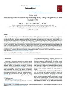
select the best possible model but to show that a “reasonable” BGVAR model outperforms many standard models in terms of forecasting accuracy. Generalized impulse response function (GIRF) An advantage of VAR and GVAR modeling is that it is useful for policy simulation through the estimation of impulse response analysis. The GIRFs are simply the derivative of shocks, and provide important information on the interdependencies between different countries. They can also indicate how one economic variable reacts over time to a shock (or exogenous impulse) in another variable within a system that involves several variables. Table 6 illustrates the specific advantage of the BGVAR in generating the GIRF, using the predictive Bayes factors (PBF) iv of Geweke and Amisano (2010) as a criterion. When compared to the VAR, BVAR, and GVAR models, the PBF favors the BGVAR model. It does so more when the forecasting horizon is extended from 1 to 2, 3, and 4 quarters ahead. This is evidence that the BGVAR model performs better in terms of out-of-sample forecasting. Therefore, an impulse response analysis from this analysis should be more credible. Having confirmed this, we report the significant GIRF effects between the countries included in our analysis in Table 7, with respect to a shock to tourist arrivals. A common trend is found among all cases with significant GIRF effects. That is, a shock in a country tends to have particularly significant effects on its border-sharing neighboring countries. For example, we can see that a shock in Cambodia will have a one-period effect on Laos, a shock in Malaysia will have a one-period effect on Thailand, and a shock in Vietnam will have a two-period effect on Laos and a one-period effect on Cambodia. This is clear evidence of the interdependency of tourism demand between neighboring countries, which can be explained by frequent crossborder social, cultural, and economic exchanges. Multi-destination visits by long-haul tourists may also have an effect. For example, an American tourist may visit Vietnam, Laos, and Cambodia during the same trip. In addition, the frequency of the significant responses a country has to a shock in another country shown in Table 7 suggests that tourism in Indonesia is the most closely interrelated with that of the other countries, while Myanmar and Vietnam appear to be the least connected to the others in the region. Interdependence can be a double-edged sword. Countries with strong tourism interdependency may both benefit and suffer from the positive and negative developments of the tourism industry of each other. The authorities in these related countries should therefore bear in mind the implications and plan their tourism development carefully. Furthermore, we examine the effects of shocks on global economic growth and each individual country’s economic growth on tourist arrivals in these countries. Figure 1 presents significant GIRF results. As Figure 1(a) suggests, an increase in global economic growth (by 10%) will boost tourism demand in the whole region of Southeast Asia (by 5-10% in each country). The region will thus collectively benefit (or suffer) from a global economic boom (or recession), at least in the short term (i.e., in the next five quarters or so). In the longer term, the responses become volatile in some countries (e.g., Malaysia, Myanmar, and the Philippines), and for a few countries (e.g., Cambodia, Indonesia, and the Philippines), the effects may even be in the opposite direction, implying fierce competition within the region and strong substitutability. Figures 1(b) to 1(e) display the significant effects of the shocks to individual countries’ GDP growth. These significant responses reveal the close interdependency among the countries, and the number of significant responses reveals the scope of the effect. It appears that the change in Indonesia’s economic growth may have the widest impact on tourist arrivals in this region; five of the other eight countries receive significant effects. In most cases, a country’s economic 10

growth has positive effects on its own tourist arrivals and those in other countries in the region, which can be explained from two perspectives. First, economic growth in a country encourages more outbound tourism from it to its neighbors. Second, economic growth in one country may have positive spill-over effects on the others, and more economic exchanges between them are likely to take place within the region, and between the region and the rest of the world, which leads to more business travel into the region and between the countries. However, in some cases (e.g., Indonesia, Cambodia, and the Philippines) negative effects on tourist arrivals are observed in the medium term (beyond eight quarters), which may be because they have a relatively unfavorable position in terms of regional competition and they become less attractive than their neighbors. Given the economic importance of tourism in these countries, their national governments and tourism authorities should consider how to improve their competitiveness. 6. Conclusion This study presents the first attempt to examine the interdependencies of tourism demand in multiple destinations based on an advanced and innovative econometric technique: the BGVAR model. Through an empirical case of international tourist flows in nine countries in Southeast Asia, we demonstrate that the BGVAR model can capture the linkages between these countries via impulse response analysis. An external shock to a key economic variable (such as GDP, CPI, or the exchange rate) in one destination has spill-over effects on the tourism demand and other variables in neighboring countries. In addition, this is the first time the BGVAR model has been applied in the tourism demand forecasting literature. This study presents empirical evidence of the superiority of the BGVAR model, in terms of its forecasting accuracy, over three alternative VAR specifications including the unrestricted VAR, GVAR, and BVAR models, and the traditional ARMA model. The BGVAR model consistently outperforms its competitors across all forecasting horizons (one to four quarters ahead), in all nine countries, based on all the forecast error measures used. The findings of this empirical study have important implications for destination management. First, the proven interdependencies among neighboring countries in the same region require their governments and destination management organizations (DMOs) to take account of the external (both global and regional) environment in their strategic planning and management. As illustrated in Figure 1, changes in the global economic climate (e.g., a global economic crisis) will have a widespread effect on the tourism industries of all countries in Southeast Asia. A regional (i.e., super-national) perspective of destination management is thus necessary. Given the competitive nature of the tourism industry within a specific geo-economic region, countries within the region should work together in terms of marketing and planning with a view to enhancing regional tourism competitiveness. ASEAN is a well-established, effective platform for such regional cooperation, and it should be used more effectively to facilitate regional tourism development, such as holding forums to exchange knowledge and experience, and organizing joint promotional campaigns in key source markets. Second, the evidence provided by impulse response analysis of the different types and degrees of response when a country is exposed to an external shock suggests that each destination should identify the types of shocks, and the countries they are most inter-dependent with. Shock- and country specific strategies can then be developed. Interdependency means that if there is a positive response to a positive shock, there will also be a negative response to a negative shock, which indicates vulnerability. Each country should capitalize on the positive spill-over effects of interdependency, while also developing contingency plans to minimize the

11

effects of a potential negative shock. A fine balance between independence and interdependence in tourism development is thus required. The impulse response analysis reveals that the tourism industries of border-sharing neighboring countries (e.g., Cambodia and Laos, and Indonesia and the Philippines) are highly interdependent and vulnerable to any shock to each other’s tourism growth. The DMOs of these countries should closely monitor their neighboring countries’ tourism development. For example, once a shock happens to the tourism industry in Cambodia (or Indonesia), a timely counter strategy in Laos (or the Philippines) should be put in place. By examining the number of significant responses to a shock a country receives, we can see that the tourism industry in Indonesia is the most vulnerable in the region, and those of Vietnam and Myanmar are the least connected with the rest of the region. Unique tourism product offers should thus be developed in Indonesia, while the priority for Vietnam and Myanmar should be to enhance their cooperation and coordination with the rest of the region and between each other, to realize the potential of regional spill-over effects. In addition, as Figure 1 illustrates, a shock to the economic growth of a country will not only affect tourist arrivals in the country but also in others in the region. The results of this study can help national governments identify the other countries that have strong economic ties with them and that deserve more attention. For example, a shock to Indonesia’s economic growth has the widest effect on regional tourist arrivals (e.g., in Singapore, Malaysia, Thailand, Cambodia, and the Philippines), so these countries should closely monitor the economic situation in Indonesia and have their scenario planning in place. Once a certain shock affects Indonesia’s economy, the other countries in the region should react in a timely fashion. Countries (e.g., the Philippines) whose tourist arrivals may be adversely affected by the economic growth of their neighbors should carefully consider how to improve their tourism competitiveness within the region. Knowledge transfer and product innovation could be key considerations in their strategic planning. Learning from neighbors’ successful experiences and capitalizing on unique strengths can be effective strategies for catching up. The shock period estimated in the BGVAR impulse response analysis (see Table 7) is also useful for tourism businesses to effectively and flexibly plan for production and employment adjustments. A more general implication is that an effective risk and crisis management strategy for a destination should combine general principles with specific procedures and approaches relevant to the types and sources of risk. Last, a systematic approach to tourism demand forecasting can more accurately and usefully support strategic planning. Given the interdependencies among destinations, forecasting future tourism trends in a destination without considering the geographical spill-over effects may lead to biased results and misinform the strategic decision making. DMOs and tourism businesses will therefore find applications of BGVAR forecasting beneficial to effective planning and strategies, particularly in an increasingly competitive environment. The empirical evidence of the superior properties of the BGVAR model and its forecasting performance, and its applicability in tourism studies, suggests that further applications of this method can be extremely useful. For example, future research may consider a truly global tourism system, and investigate the interdependencies of tourist flows on a global scale. After the UK’s European Union membership referendum, the pound has fallen significantly, so the BGVAR model could be an effective tool for quantifying the effect on tourism demand not only in the UK, but also in other European countries and the rest of the world. 12

To conclude, we acknowledge some limitations of the present study. As with most tourism forecasting, in this research, we take a real-world case study approach to demonstrate the applicability and effectiveness of the BGVAR model in tourism forecasting. The intention in this study was not to draw a generalized conclusion. The forecasting performance of the BGVAR model can be further examined in other empirical cases. The data availability limitations meant we focused on a short sample period. Future studies may also consider extending the data and examining the forecasting accuracy of the BGVAR model over longer forecasting horizons. In addition, we also note that raw data without seasonal adjustment would have more direct practical implications. With seasonally adjusted data, however, the findings of the study are still valid, and we have been able to achieve the main objective of the study. Future research can further consider tourism seasonality in BGVAR modeling and forecasting.

References Abel, A. B., B. Bernanke, and D. D. Croushore. 2008. Macroeconomics (6th edition). Boston/London: Pearson/Addison Wesley. Berg, T. O., and S. R. Henzel. 2015. “Point and Density Forecasts for the Euro Area Using Bayesian VARs.” International Journal of Forecasting 31: 1067-95. Boschi, M. 2012. “Long- and Short-Run Determinants of Capital Flows to Latin America: A Long-Run Structural GVAR Model.” Empirical Economics 43 (3): 1041-71. Calantone, R. J., C. A. Di Benedetto, and D. Bojanic. 1987. “A Comprehensive Review of the Tourism Forecasting Literature.” Journal of Travel Research 26 (2): 28-39. Cao, Z., G. Li, and H. Song. 2017. “Modeling the Interdependence of International Tourism Demand: The Global VAR Approach.” Annals of Tourism Research 67 (1): 1-13. Caraiani, P. 2010. “Forecasting Romanian GDP Using a BVAR Model.” Romanian Journal of Economic Forecasting 4: 76-87. Carriero, A., T. G. Clark, and M. Marcellino. 2015. “Bayesian VARs: Specification Choices and Forecast Accuracy.” Journal of Applied Econometrics 30 (1): 46-73. Carriero, A., G. Kapetanios, and M. Marcellino. 2009. “Forecasting Exchange Rates with a Large Bayesian VAR.” International Journal of Forecasting 25: 400-17. Carriero, A., G. Kapetanios, and M. Marcellino. 2012. “Forecasting Government Bond Yields with Large Bayesian Vector Autoregressions.” Journal of Banking and Finance 36: 202647. Chudik, A., and M. Fratzscher. 2011. “Identifying the Global Transmission of the 2007-2009 Financial Crisis in a GVAR Model.” European Economic Review 55 (3): 325-39. Chudik, A., and R. Straub. 2010. “Size, Openness, and Macroeconomic Interdependence.” Working Paper Series 1072, European Central Bank. http://www.ecb.europa.eu/pub/pdf/scpwps/ecbwp1172.pdf. Cortés-Jiménez, I., R. Durbarry, and M. Pulina. 2009. “Estimation of Outbound Italian Tourism Demand: A Monthly Dynamic EC-LAIDS Model.” Tourism Economics 15: 547-65. Dees, S., F. D. Mauro, M. H. Pesaran, and L. V. Smith. 2007. “Exploring the International Linkages of the Euro Area: A Global VAR Analysis.” Journal of Applied Econometrics 22 (1): 1-38. Diebold, F. X., and R. Mariano. 1995. “Comparing Predictive Accuracy.” Journal of Business and Economic Statistics 13: 253-265. Doan, T. A., R. B. Litterman, and C. Sims. 1984. “Forecasting and Conditional Projection Using Realistic Prior Distributions.” Econometric Reviews 3: 1-100. 13

Feller, W. 1966. “Infinitely Divisible Distributions and Bessel Functions Associated with Random Walks.” SIAM Journal on Applied Mathematics 14 (4): 864-75. Galesi, A., and M. J. Lombardi. 2009. “External Shocks and International Inflation Linkages: A Global VAR Analysis.” Working Paper Series 1062, European Central Bank. http://www.ecb.europa.eu/pub/pdf/scpwps/ecbwp1062.pdf. Galesi, A., and S. Sgherri. 2009. “Regional Financial Spillovers across Europe: A Global VAR Analysis.” IMF Working Papers 09/23, International Monetary Fund. http://www.imf.org/external/pubs/ft/wp/2009/wp0923.pdf. Geweke, J., and Amisano, G. 2010. “Comparing and evaluating Bayesian predictive distributions of asset returns.” International Journal of Forecasting 26: 216-230. Girolami, M., and B. Calderhead. 2011. “Riemann Manifold Langevin and Hamiltonian Monte Carlo Methods.” Journal of the Royal Statistical Society, Series B 73 (2):123-214. Greenwood-Nimmo, M., V. H. Nguyen, and Y. Shin. 2012. “Probabilistic Forecasting of Output Growth, Inflation and the Balance of Trade in A GVAR Framework.” Journal of Applied Econometrics 27 (4): 554-73. Hamilton, J. D. 1994. Time Series Analysis. Princeton: Princeton University Press. Harvey, D. I., S. J. Leybourne, and P. Newbold. 1997. “Testing the Equality of Prediction Mean Squared Errors.” International Journal of Forecasting 13: 281-291. Hitchcock, M., V. P. King, and M. Parnwell. 2008. “Introduction: Tourism in Southeast Asia Revisited.” In Tourism in Southeast Asia: Challenges and New Directions, edited by M. Hitchcock, V. P. King, and M. Parnwell, 1-42. Copenhagen, NISA Press. Hiebert, P., and I. Vansteenkiste. 2010. “International Trade, Technological Shocks and Spillovers in the Labour Market: A GVAR Analysis of the US Manufacturing Sector.” Applied Economics 42 (24): 3045-66. Huang, A., and M. P. Wand. 2013. “Simple Marginally Noninformative Prior Distributions for Covariance Matrices.” Bayesian Analysis 8 (2): 439-52. International Monetary Fund 2014. World Economic Outlook—Recovery Strengthens, Remains Uneven. Washington, April 2015. Kadiyala, K. R., and S. Karlsson. 1997. “Numerical Methods for Estimation and Inference in Bayesian VAR-Models.” Journal of Applied Econometrics 12: 99-132. Koop, G. 2013, “Forecasting with Medium and Large Bayesian VARs.” Journal of Applied Econometrics 28: 177-203. Koop, G., and D. Korobilis. 2013. “Large Time-Varying Parameter VARs.” Journal of Econometrics, In Press. Koop, G., M. H. Pesaran, and S. M. Potter. 1996. “Impulse Response Analysis in Nonlinear Multivariate Models.” Journal of Econometrics 74 (1): 119-47. Li, G., H. Song, and S. F. Witt. 2004. “Modeling Tourism Demand: A Dynamic Linear AIDS Approach.” Journal of Travel Research 43 (2): 141-150. Li, G., H. Song, and S. F. Witt. 2005. “Recent Developments in Econometric Modeling and Forecasting”. Journal of Travel Research, 44 (1): 82-99. Li, G., K. K. F. Wong, H. Song, and S. F. Witt. 2006. “Tourism Demand Forecasting: A Time Varying Parameter Error Correction Model.” Journal of Travel Research 45 (2): 175-85. Litterman, R. B. 1986. “Forecasting with Bayesian Vector Autoregressions: Five Years of Experience.” Journal of Business and Economic Statistics 4: 25-38. Massidda, C., and P. Mattana. 2013. “A SVECM Analysis of the Relationship between International Tourism Arrivals, GDP and Trade in Italy.” Journal of Travel Research 52 (1): 93-105. N’Diaye, P., and A. Ahuja. 2012. “Trade and Financial Spillover on Hong Kong SAR from a Downturn in Europe and Mainland China.” IMF Working Papers 12/81, International Monetary Fund. http://www.imf.org/external/pubs/ft/wp/2012/wp1281.pdf. 14

Nowak, J. J., M. Sahli, and I. Cortes-Jimenez. 2007. “Tourism, Capital Good Imports and Economic Growth: Theory and Evidence for Spain.” Tourism Economics 13 (4): 515-36. Pacific Asia Travel Association (PATA). 2015. Quarterly Tourism Monitor 2014. Bangkok, PATA. Pan, B., and Y. Yang. 2017, “Forecasting Destination Weekly Hotel Occupancy with Big Data.” Journal of Travel Research 56 (7): 957-970. Pesaran, M. H., L. V. Smith, and R. P. Smith. 2007. “What if the UK or Sweden Had Joined the Euro in 1999? An Empirical Evaluation Using a Global VAR.” International Journal of Finance & Economics 12 (1): 55-87. Pesaran, M. H., T. Schuermann, and L. V. Smith. 2009. “Forecasting Economic and Financial Variables with Global VARs.” International Journal of Forecasting 25 (4): 642-75. Pesaran, M. H., T. Schuermann, and S. M. Weiner. 2004. “Modeling Regional Interdependencies Using a Global Error-Correcting Macroeconometric Model.” Journal of Business and Economic Statistics 22 (2): 129-62. Pesaran, M. H. and Y. Shin. 1998. “Generalized Impulse Response Analysis in Linear Multivariate Models.” Economics Letters 58 (1): 17-29. Rebucci, A., and M. Ciccarelli. 2003. “Bayesian VARs: A Survey of the Recent Literature with an Application to the European Monetary System.” IMF Working Paper WP/03/102, International Monetary Fund. Schubert, S. F., J. G. Brida, and W. A. Risso. 2011. “The Impacts of International Tourism Demand on Economic Growth of Small Economies Dependent on Tourism.” Tourism Management 32: 377-85. Seo, J. H., S. Y. Park, and S. Boo. 2010. “Interrelationships among Korean Outbound Tourism Demand: Granger Causality Analysis.” Tourism Economics 16 (3): 597-610. Song, H., and S. F. Witt. 2006. “Forecasting International Tourist Flows to Macau.” Tourism Management 27 (2): 214-24. Song, H., L. Dwyer, G. Li, and Z. Cao. 2012. “Tourism Economics Research: A Review and Assessment.” Annals of Tourism Research 39 (3): 1653-82. Stock, J. H., and M. W. Watson. 2012. Introduction to Econometrics (3rd Ed., Global Ed.). Boston, Mass.; London: Pearson. Torraleja, F. A. G., A. M. Vázquez, and M. J. B. Franco. 2009. “Flows into Tourist Areas: An Econometric Approach.” International Journal of Tourism Research 11 (1): 1-15. Tribe, J. 2011. Economics of Recreation, Leisure and Tourism. London: Taylor and Francis. Tsionas, E. G., K. N. Konstantakis, and P. G. Michaelides. 2016. “Bayesian GVAR with Kendogenous Dominants & Input–Output Weights: Financial and Trade Channels in Crisis Transmission for BRICs.” Journal of International Financial Markets, Institutions and Money 42: 1-26. United Nations World Tourism Organization. 2014. UNWTO Tourism Highlights 2014 Edition. Madrid: UNWTO. Uysal, M., and J. L. Crompton. 1985. “An Overview of Approaches Used to Forecast Tourism Demand.” Journal of Travel Research 23 (4): 7-15. Vansteenkiste, I., and P. Hiebert. 2011. “Do House Price Developments Spillover across Euro Area Countries? Evidence from a Global VAR.” Journal of Housing Economics 20 (4): 299314. West, M. 1987. “On Scale Mixtures of Normal Distributions.” Biometrika 74 (3): 646-48. Witt, S. F., H. Song, and P. Louvieris. 2003. “Statistical Testing in Forecasting Model Selection.” Journal of Travel Research 42 (2): 151-158. Wong, K. K. F., H. Song, and K. S. Chon. 2006. “Bayesian Models for Tourism Demand Forecasting.” Tourism Management 27: 773-80.

15

World Travel and Tourism Council. 2011. The Review 2011. http://www.wttc.org/site_media/uploads/downloads/WTTC_Review_2011.pdf. Wu, D. C., G. Li, and H. Song. 2011. “Analyzing Tourist Consumption: A Dynamic Systemof-Equations Approach.” Journal of Travel Research 50 (1): 46-56. Wu, D. C., H. Song, and S. Shen. 2017. “New Developments in Tourism and Hotel Demand Modeling and Forecasting.” International Journal of Contemporary Hospitality Management 29 (1): 507-529. Yang, Y., T. J. Fik, and H. Zhang. 2017. “Designing a Tourism Spillover Index Based on Multidestination Travel: A Two-Stage Distance-Based Modeling Approach.” Journal of Travel Research 56 (3): 317-333.

16

Table 1. Forecasting Performance, RMSE Cambodia VAR BVAR GVAR BGVAR ARMA Indonesia VAR BVAR GVAR BGVAR ARMA Laos VAR BVAR GVAR BGVAR ARMA Malaysia VAR BVAR GVAR BGVAR ARMA Myanmar VAR BVAR GVAR BGVAR ARMA Philippines VAR BVAR GVAR BGVAR ARMA Singapore VAR BVAR GVAR BGVAR ARMA

1-quarter ahead

2-quarter ahead

3-quarter ahead

4-quarter ahead

0.014 0.012 0.011 0.007 0.009

0.022 0.019 0.013 0.009 0.012

0.039 0.025 0.019 0.011 0.014

0.051 0.037 0.031 0.017 0.021

0.019 0.018 0.012 0.005 0.009

0.025 0.020 0.017 0.007 0.013

0.041 0.035 0.028 0.012 0.015

0.057 0.051 0.044 0.017 0.021

0.005 0.003 0.003 0.001 0.004

0.012 0.009 0.008 0.004 0.007

0.019 0.011 0.010 0.007 0.011

0.026 0.022 0.019 0.009 0.020

0.008 0.007 0.004 0.002 0.007

0.013 0.012 0.010 0.005 0.008

0.017 0.013 0.011 0.007 0.009

0.022 0.020 0.018 0.010 0.014

0.014 0.010 0.010 0.007 0.010

0.018 0.015 0.014 0.009 0.012

0.025 0.021 0.019 0.011 0.014

0.031 0.029 0.025 0.016 0.021

0.018 0.014 0.010 0.007 0.012

0.023 0.019 0.014 0.010 0.015

0.027 0.023 0.020 0.015 0.018

0.033 0.028 0.023 0.019 0.023

0.005 0.004 0.003 0.001 0.004

0.012 0.010 0.007 0.003 0.010

0.018 0.015 0.010 0.006 0.012

0.023 0.019 0.015 0.008 0.015

17

Thailand VAR BVAR GVAR BGVAR ARMA

0.013 0.010 0.009 0.004 0.009

0.017 0.013 0.010 0.007 0.011

0.023 0.017 0.014 0.009 0.013

0.029 0.021 0.018 0.010 0.015

Vietnam VAR 0.016 0.019 0.022 0.034 BVAR 0.012 0.017 0.018 0.021 GVAR 0.007 0.012 0.013 0.019 BGVAR 0.005 0.008 0.009 0.011 ARMA 0.009 0.011 0.012 0.018 Notes: VAR is the simple VAR model whose lag order is selected using the Schwarz criterion. BVAR is a Bayesian VAR model with a Minnesota prior. GVAR is a global VAR model estimated using sampling-theory techniques. BGVAR is the Bayesian global VAR model. ARMA is an autoregressive-moving average model whose forecasts are univariate. Its orders are selected using the AIC criterion.

Table 2. Forecasting Performance, MAE Cambodia VAR BVAR GVAR BGVAR ARMA Indonesia VAR BVAR GVAR BGVAR ARMA Laos VAR BVAR GVAR BGVAR ARMA Malaysia VAR BVAR GVAR BGVAR ARMA Myanmar VAR BVAR

1-quarter ahead

2-quarter ahead

3-quarter ahead

4-quarter ahead

0.017 0.013 0.009 0.005 0.011

0.019 0.014 0.011 0.005 0.012

0.022 0.019 0.012 0.007 0.009

0.027 0.022 0.013 0.011 0.017

0.021 0.017 0.009 0.004 0.007

0.025 0.020 0.012 0.005 0.013

0.028 0.022 0.014 0.007 0.011

0.033 0.025 0.017 0.009 0.012

0.020 0.018 0.007 0.001 0.005

0.025 0.020 0.009 0.002 0.013

0.031 0.022 0.012 0.003 0.009

0.037 0.027 0.015 0.005 0.013

0.019 0.013 0.005 0.002 0.011

0.023 0.015 0.007 0.004 0.010

0.028 0.017 0.009 0.005 0.012

0.032 0.019 0.013 0.009 0.013

0.014 0.011

0.018 0.014

0.019 0.017

0.025 0.022

18

GVAR BGVAR ARMA Philippines VAR BVAR GVAR BGVAR ARMA Singapore VAR BVAR GVAR BGVAR ARMA

0.007 0.006 0.009

0.011 0.007 0.010

0.013 0.009 0.011

0.017 0.010 0.014

0.017 0.013 0.009 0.005 0.008

0.022 0.015 0.015 0.007 0.009

0.027 0.021 0.017 0.010 0.012

0.032 0.028 0.019 0.013 0.018

0.017 0.010 0.007 0.003 0.009

0.022 0.015 0.012 0.006 0.012

0.028 0.019 0.017 0.009 0.014

0.031 0.022 0.021 0.011 0.015

Thailand VAR 0.018 0.022 0.027 0.033 BVAR 0.013 0.015 0.017 0.021 GVAR 0.007 0.009 0.019 0.023 BGVAR 0.003 0.005 0.007 0.009 ARMA 0.007 0.008 0.011 0.012 Vietnam VAR 0.019 0.023 0.027 0.029 BVAR 0.015 0.018 0.021 0.025 GVAR 0.009 0.013 0.017 0.022 BGVAR 0.003 0.005 0.007 0.010 ARMA 0.007 0.009 0.011 0.015 Notes: VAR is the simple VAR model whose lag order is selected using the Schwarz criterion. BVAR is a Bayesian VAR model with a Minnesota prior. GVAR is a global VAR model estimated using sampling-theory techniques. BGVAR is the Bayesian global VAR model. ARMA is an autoregressive-moving average model whose forecasts are univariate. Its orders are selected using the AIC criterion.

19

Table 3. Forecasting Performance, MAPE 1-quarter ahead

2-quarter ahead

3-quarter ahead

4-quarter ahead

VAR BVAR GVAR BGVAR ARMA Indonesia

1.80% 1.00% 1.50% 0.30% 1.70%

2.30% 1.40% 1.10% 0.50% 2.00%

3.20% 2.10% 1.70% 0.70% 1.30%

4.10% 2.90% 3.00% 0.90% 1.70%

VAR BVAR GVAR

2.20% 1.70% 1.10%

2.90% 2.50% 1.30%

4.00% 3.10% 1.90%

5.50% 4.40% 2.60%

BGVAR

0.20%

0.40%

0.80%

0.80%

ARMA

1.20%

1.80%

2.30%

3.10%

VAR BVAR GVAR BGVAR ARMA Malaysia

1.40% 0.90% 0.70% 0.20% 1.20%

2.70% 1.70% 1.20% 0.30% 1.80%

3.10% 2.20% 1.70% 0.50% 2.00%

5.00% 3.00% 2.20% 0.70% 2.50%

VAR BVAR GVAR BGVAR ARMA Myanmar

1.40% 0.90% 0.70% 0.20% 1.20%

2.70% 1.70% 1.20% 0.30% 1.80%

3.10% 2.20% 1.70% 0.50% 2.00%

5.00% 3.00% 2.20% 0.70% 2.50%

VAR BVAR GVAR BGVAR ARMA Philippines

2.30% 1.90% 1.40% 0.30% 1.80%

3.20% 2.50% 1.70% 0.30% 1.30%

4.20% 2.70% 1.90% 0.50% 1.40%

5.50% 3.30% 2.10% 0.60% 2.10%

VAR BVAR GVAR BGVAR

2.80% 1.80% 1.20% 0.40%

3.40% 2.40% 1.50% 0.50%

4.40% 2.70% 2.50% 0.50%

5.30% 3.20% 2.90% 0.90%

ARMA Singapore

1.20%

1.00%

1.70%

2.40%

Cambodia

Laos

20

VAR BVAR GVAR BGVAR ARMA Thailand VAR BVAR GVAR BGVAR ARMA Vietnam

2.10% 1.40% 0.80% 0.20% 1.20%

3.30% 2.20% 1.40% 0.40% 2.10%

4.50% 3.00% 1.70% 0.50% 2.30%

5.50% 3.20% 2.50% 0.70% 2.70%

2.40% 1.80% 1.10% 0.20% 1.30%

3.80% 2.50% 1.70% 0.40% 2.50%

4.10% 2.90% 2.10% 0.50% 3.10%

4.90% 3.20% 2.80% 0.70% 2.70%

VAR 2.20% 2.80% 4.40% 6.60% BVAR 1.80% 2.20% 2.60% 3.00% GVAR 1.10% 1.80% 2.20% 2.80% BGVAR 0.30% 0.40% 0.50% 1.00% ARMA 1.80% 2.30% 2.70% 2.40% Sample average VAR 2.07% 3.01% 3.89% 5.27% BVAR 1.47% 2.12% 2.61% 3.24% GVAR 1.07% 1.43% 1.93% 2.57% BGVAR 0.26% 0.39% 0.56% 0.78% ARMA 1.40% 1.84% 2.09% 2.46% Notes: VAR is the simple VAR model whose lag order is selected using the Schwarz criterion. BVAR is a Bayesian VAR model with a Minnesota prior. GVAR is a Global VAR model estimated using sampling-theory techniques. BGVAR is the Bayesian Global VAR model.

21

Table 4. Diebold-Mariano Tests for Forecast Equivalence between BGVAR and GVAR Models 1-quarter

2-quarter

3-quarter

4-quarter

Cambodia

0.0000

0.0000

0.0000

0.0000

Indonesia

0.0000

0.0002

0.0000

0.0000

Laos

0.0000

0.0000

0.0000

0.0000

Malaysia

0.0021

0.0012

0.0000

0.0000

Myanmar

0.0044

0.0005

0.0000

0.0000

Philippines

0.0000

0.0010

0.0000

0.0000

Singapore

0.0015

0.0002

0.0000

0.0000

Thailand

0.0022

0.0011

0.0000

0.0000

Vietnam

0.0000

0.0000

0.0000

0.0000

Note: The table reports the p-values of the Diebold and Mariano (1995) test. The test statistic d follows, asymptotically, the N(0,1) distribution. The test statistic is S1  , where T 1 2 fˆ (0) d

T

{d t , t  1,..., T } is a series of losses with the forecast horizon T, d  T 1 t 1 dt and fˆd (0) is a consistent estimate of the spectral density at zero frequency.

Table 5. Results of Prior Sensitivity Analysis (for All Countries) Competing model

Frequency of Competing model Frequency of BGVAR forecasts BGVAR forecasts with lower RMSE with lower MAE VAR 96.7% VAR 97.7% BVAR 90.3% BVAR 96.4% ARMA(p,q) 99.1% ARMA (p,q) 99.0% Benchmark BGVAR 77.4% Benchmark BGVAR 63.5% Notes: The orders p, q of ARMA processes are selected using the BIC criterion and are estimated in-sample using maximum likelihood. Here the ARMA (p,q) scheme is applied to each variable. RMSE and MAE refer to four quarters ahead. Note that we also computed the AIC (and other model selection measures), which typically provides the same or a larger number of lags. The forecasting performance based on the stated forecast accuracy measures was never better than the results we achieved.

22

Table 6. Predictive Bayes Factors in Favor of BGVAR against VAR, BVAR, and GVAR Models 1-quarter-ahead 2-quarter-ahead 3-quarter-ahead 4-quarter-ahead VAR

17.225

24.761

33.154

57.045

BVAR

8.332

19.301

27.515

44.021

GVAR

71.230

121.44

217.32

281.90

Table 7. GIRF Effects of Tourist Arrivals between the Various Countries Covered in the Sample Country of Country of Response and Period Shock Cambodia Laos, 1 period Indonesia Philippines 1 period, Thailand 1 period Laos Cambodia, 1 period Malaysia Indonesia, periods 1 and 2 Myanmar Thailand 1 period Philippines Indonesia 1 period Singapore Philippines 1 period Indonesia 1 period Thailand Indonesia 1 period, Singapore 1 period Vietnam Laos, periods 1 and 2, Cambodia 1 period *Numbers in parentheses are the standard deviations.

23

Total GIRF Effect 0.130 (0.051) 0.072 (0.012) 0.044 (0.015) 0.315 (0.021) 0.414 (0.009) 0.137 (0.025) 0.045 (0.012) 0.212 (0.045) 0.316 (0.032) 0.175 (0.044) 0.503 (0.041) 0.483 (0.060)

Figure 1. Generalized Impulse Responses of Shocks to Global and National Economic Growth Figure 1(a) A Shock to Global GDP Growth

0.1

0.2

0.2

Cambodia

Indonesia

0

-0.1

0

0

5

10

0.1

-0.2

0

0

10

5

10

0.2

0

0

5

10

-0.1

0

Thailand

10

0

5

10

0.2 Vietnam

0.1

5

10

0

Singapore 0.1

5 Philippines

0.2

0

0

0.1

0.05

0

-0.2

Myanmar

0.05

0

5

0.1 Malaysia

0

Laos

0.1

0

5

24

10

0

0

5

10

Figure 1(b) A Shock to Singapore’s GDP Growth

0.2 Singapore 0.1

0

0

1

2

3

4

5

6

7

8

9

10

0.1 Philippines 0

-0.1

0

1

2

3

4

5

6

7

8

9

10

0.2 Thailand 0

-0.2

0

1

2

3

4

5

25

6

7

8

9

10

Figure 1(c) A Shock to the Philippines’ GDP Growth

0.15

0.15 Philippines

Singapore

0.1

0.1

0.05

0.05

0

0

-0.05

0

5

10

0.15

-0.05

0

5

0.15 Thailand

Indonesia

0.1

0.1

0.05

0.05

0

0

-0.05

10

0

5

10

-0.05

26

0

5

10

Figure 1(d) A Shock to Malaysia’s GDP Growth

0.15

0.2 Malaysia

Singapore

0.1

0.15

0.05

0.1

0

0.05

-0.05

0

5

0

10

0.15

0

5

0.2 Philippines

Thailand

0.1

0.15

0.05

0.1

0

0.05

-0.05

10

0

5

0

10

27

0

5

10

Figure 1(e) A Shock to Indonesia’s GDP Growth

0.1

0.2 Indonesia

Singapore

0

-0.1

0.1

0

5

0

10

0.2

0

5

0.2 Malaysia

Philippines 0

-0.2

0.1

0

5

0

10

0.1

0

5

10

0.1 Thailand

Cambodia

0.05

0

10

0

0

5

10

-0.1

28

0

5

10

Appendix 1: Prior of Huang and Wand (2013) The proposed family of Huang and Wand’s (2013) prior is defined as follows:  | a1 ,...a p ~ IW A ,  p  1 , where IW denotes the inverted Wishart distribution,

 p p 





A  2 diag a11 ,..., a p1 , a k ~ IG

 , , k  1,.., p 1 2

1 A k2

where p = Nm is the dimensionality of Σ. We k/2





note the density of the Wishart W k , S  is: p  S exp  12 trS , k  0 , and , S are positive definite matrices. In this construction  , A1 ,..., A p are positive parameters that we set 1

to 1 and 0.1, respectively. Large values of A1 ,..., Ap imply weakly informative priors on the standard deviations, while the choice

 2

leads to uniform priors on the correlation 

.      The marginal distribution of each correlation coefficient is p   1    , 1  

coefficients. The explicit form of the prior is p  

  2 p  / 2

k 1

  p  / 2

1

1 Ak2

kk

2 ij

ij

 1 2

ij

1

. The marginal distribution of each standard deviation follows a half-t distribution with parameters  , Ak , that is:  ii2 | a i ~ IW  , 2a , and independently a i ~ IG 12 , A1 , i  1,..., p .



i

2 i



The main characteristics of the distribution that make it particularly appealing in MCMC computation are that its conditional distribution is still an inverse Wishart (conditional on the ai s) and the posterior conditionals of ai s are inverse-Gamma distributions (Huang and Wand 2013).

29

Appendix 2: Posterior Computation We use a Girolami and Calderhead (2011, GC) algorithm to update draws for a parameter  . The algorithm uses local information about both the gradient and the Hessian of the logposterior conditional of  at the existing draw. The GC algorithm is started at the first-stage GMM estimator and MCMC is run until convergence. The GC algorithm is found to have vastly superior performance relative to the standard MH algorithm, and the autocorrelations are much smaller. Suppose L    log p   X  is used to denote for simplicity the log posterior of  . We define G    est cov  log p  X   

(12)

As the empirical counterpart of 2    

G o     E Y 

log p  X   

(13)

The Langevin diffusion is given by the following stochastic differential equation: d   t   12 % L   t  dt  d B  t 

(14)

where 1 % L   t    G   t   % L   t 

(15) is the so called “natural gradient” of the Riemann manifold generated by the log posterior. The elements of the Brownian motion are G 1   t  dB i  t   G   t  1 2

K

 j 1

    



G 1  t ij  G   t  1 2  dt

(16)



 G  t dB  t   i The discrete form of the stochastic differential equation provides the following proposal: K 

  o 2 1  o   o     1  o  %i  i  2 G    L   i    j1 G   2



2

 2



K    j 1 





G 1   o   tr G 1   o   ij

 G  a o  



 j

     







i

G o  

 j





G1  o  

 ij



G 1   o  o 

 i

   o      G 1  o  o  i

where  o is the current draw. The proposal density is   q %  o   N %  2G 1  o   

K 







(17)

and convergence to the invariant distribution is ensured by using the standard form MetropolisHastings probability  p %  Y q  o  %  min 1 (17)  % o o  p    Y q   a  

 

  

30



Appendix 3: Results of Prior Sensitivity Analysis by Country Table A1. Frequencies of BGVAR Forecasts with Lower RMSE and Lower MAE Frequency of VAR BVAR ARMA(p,q) Benchmark BGVAR forecasts: BGVAR With lower RMSE Cambodia 93.2% 92.5% 99.1% 41.5% Indonesia 95.5% 90.0% 99.7% 62.5% Malaysia 99.4% 88.4% 98.5% 55.7% Myanmar 94.7% 90.5% 98.0% 73.2% Philippines 96.2% 97.2% 98.7% 70.0% With lower MAE Cambodia 99.0% 94.0% 98.2% 77.3% Indonesia 98.3% 95.4% 99.0% 60.0% Malaysia 97.5% 96.4% 99.7% 45.3% Myanmar 98.5% 97.3% 100% 33.2% Philippines 99.2% 98.7% 100% 65.0% Notes: The orders p, q of ARMA processes are selected using the BIC criterion and are estimated in-sample using maximum likelihood. Here, the ARMA (p,q) scheme is applied to each variable. RMSE and MAE refer to four quarters ahead. The results for other countries were similar.

Table A2. Percentage Forecast Accuracy Differences between the Benchmark BGVAR and the Best Performing BGVAR Country % difference RMSE % difference MAE Cambodia 7.3% 4.5% Indonesia 5.1% 3.3% Malaysia 11.5% 9.4% Myanmar 8.2% 7.0% Philippines 7.2% 4.3% Singapore 4.5% 3.7% Thailand 3.3% 2.5% Vietnam 6.0% 4.2% Laos 15.3% 8.2% Notes: The orders p, q of ARMA processes are selected using the BIC criterion and are estimated in-sample using maximum likelihood. RMSE and MAE refer to four quarters ahead. The best performing BGVAR model is the one with a prior that yields the minimum possible RMSE or MAE. The results for other countries were similar. i

For simplicity, we omit deterministic trends and constants. In the following empirical study, consistent with previous tourism demand studies, constants are included in the specified model and deterministic trends are excluded. ii For a single country see Kadiyala and Carlsson (1997, 101) and Koop and Korobilis (2013). iii The models are estimated using the data up to 2013Q2 and the remaining sample (i.e., the last four quarters from 2013Q3 to 2014Q2) are reserved for dynamic forecasting and forecast accuracy evaluation. iv The PBF is a ratio of two marginal likelihoods when we predict out of sample (see Formula 7 of Geweke and Amisano 2010).

31