Oct 2, 2015 - AbstractâIn this paper, the implementation of a variable stiffness joint actuated by a couple of twisted string actuators in antagonistic ...
2015 IEEE/RSJ International Conference on Intelligent Robots and Systems (IROS) Congress Center Hamburg Sept 28 - Oct 2, 2015. Hamburg, Germany
Modeling and Identification of a Variable Stiffness Joint Based on Twisted String Actuators G. Palli, M. Hosseini, L. Moriello and C. Melchiorri DEI - Universit`a di Bologna, Viale Risorgimento 2, Bologna, Italy Abstract— In this paper, the implementation of a variable stiffness joint actuated by a couple of twisted string actuators in antagonistic configuration is presented. The twisted string actuation system is particularly suitable for very compact and light-weight robotic devices, like artificial limbs and exoskeletons, since it renders a very low apparent inertia at the load side, allowing the implementation of powerful tendon-based driving systems, using small-size DC motors characterized by high speed, low torque and very limited inertia. After the presentation of the basic properties of the twisted string actuation system, the way how they are used for the implementation of a variable stiffness joint is discussed. A simple PID-based motorside algorithm for controlling simultaneously both the joint stiffness and position is discussed, then the identification of the system parameters is performed on an experimental setup for verifying the proposed model and control approach. Index Terms— Variable Stiffness, Twisted String Actuation, Tendon Transmission Systems.
I. I NTRODUCTION The Twisted String Actuation (TSA) concept [1], [2] represents a very interesting design solution for the implementation of very compact and low cost linear transmission systems. Indeed, with an proper choice of the strings parameters (in particular the radius and length), it is possible to easily satisfy the usually tight requirements for the implementation of miniaturized and highly-integrated mechatronic devices. As a proof of its benefits and advantages, the TSA has been already successfully used for the implementation of different robotic devices like robotic hands [3], [4], exoskeletons [5] and tensegrity robots for space applications [6]. The mathematical model of the TSA and, in particular, the analysis of its force/position characteristic and of the resulting transmission stiffness has been investigated in [2]. Recently, the TSA model has also been improved taking into account the characteristics of different type of strings and a non constant string radius in [7] and its stiffness variability [8]. On the other hand, a relevant research interested all over the world is devoted to the implementation of Variable Stiffness Joints (VSJs) [9] because they allow to solve several safety issues related to the interaction of robots with unknown environments and humans. Many different VSJ implementations can be found in literature, the most noticeable are the VSA-II [10], where the variable stiffness is obtained by coupling two electric motors to the joint through a belt and a pretensioning system, the DLR VS-Joint [11] where the circular spline of the harmonic drive is connected to the joint frame by a modulated spring, the IIT Pneumatic This activity has been supported by the University of Bologna, with the “FARB Linea 2” funding action.
978-1-4799-9994-1/15/$31.00 ©2015 IEEE
Motor B Joint
Transmission B Tendon θB
θJ
FB FA θA Tendon Transmission A Motor A
Fig. 1. Schematic representation of the rotative joint with two twisted string transmission systems.
Joint [12] actuated by McKibben motors, the AwAS-II [13] based on the moving pivot concept and the Energy-Efficient Variable Stiffness Actuators [14] developed by the Twente University. Recently, Vanderborght et al. published a review of different VSJ implementations [15]. In this paper, the TSA is used for the implementation of a VSJ. The system is composed by a couple of TSA in antagonistic configuration connected to a rotating link, as shown is the scheme reported in Fig. 1. The intrinsic nonlinearity and configuration-dependent stiffness of the TSA [2] is exploited for this purposes. The dynamic model of the VSJ and a simple PID-based controller for the regulation of both the joint position and stiffness are described, then the identification of the system parameters has been carried out to verify the model and the characteristics of the VSJ. The paper reports also the preliminary activity for the experimental evaluation of the proposed controller. II. M ODELING
OF THE
TSA
The TSA is based on a very simple principle: a couple of strings are connected in parallel on one end to a rotative electrical motor and on the other end to the load to be actuated. The rotation imposed to the strings by the electrical motor reduces their length, generating a linear motion at the load side. For the modeling of the TSA, we assume that the two strings form an ideal helix of constant radius r along the whole range of the motor angular position θ. The kinematic relationship between the motor angle and the load position can be easily derived from the geometry of the helix formed by the strings which implies the following straightforward relations: p L = θ 2 r 2 + p2 , (1) p θr θr , cos α = , tan α = , (2) sin α = L L p
1757
where α is the helix slope, L is the strand length and p is the length of the transmission system or, in other words, the load relative position wrt the motor. Note that eq. (1) can be easily obtained by “unwrapping” the helix of total length L and radius r and applying Pythagoras’ theorem to the resulting triangle. From eqs. (1) and (2) it follows that: L˙ = p˙ cos α + θ˙ r sin α.
(3)
In this analysis, the strings are assumed to act as linear springs, with the capability of resisting tensile (positive) forces only. With respect to the unloaded length L0 , the total length of a string L changes according to the fiber tension Fi and the string stiffness K (normalized with respect to the length unit), i.e. � K K �p 2 (4) p + r 2 θ 2 − L0 Fi = (L − L0 ) = L0 L0
implementation, conventional DC motors are used to drive the TSAs. Since the electric dynamics is usually very fast in comparison to the other effects and then it can be neglected, a simplified dynamic model for the DC motors is assumed. Taking into account the symmetry of the actuation system, in the following we will distinguish the two actuators by using the subscript A and B respectively. Moreover, the length of the transmission in the zero joint position is called p0 , and the maximum transmission length is limited by the controller to limit the joint motion range into the interval [−60, 60] deg. Assuming a certain minimum tension force of the TSA and considering inextensible tendons for the connection with the joint, it follows from the scheme in Fig. 1 that the length of the two TSAs pA and pB can be computed as pA = p0 − rj θj pB = p0 + rj θj
(9) (10)
where r is the string radius, θ is the motor angle and p is the resulting length of the transmission system. It is worth noticing from (4) that thepstring acts as a spring whose deformation is defined as p2 + r2 θ2 − L0 and, therefore, can be modulated through the motor angular position θ. It follows that the transmission length p is given by s � �2 Fi p = L20 1 + − θ 2 r2 (5) K
where θj and rj are the link rotation angle and the link pulley radius. Finally, the link dynamics can be modeled considering the equilibrium of the forces exerted by the two TSAs on the link pulley. It results that the complete joint dynamic model can be written as
The external torque τL provided by the motor and the load force FL can be derived from (4) and by the geometrical considerations on the system: ! L0 θ r2 K (6) 1− p τL (θ, p) = 2 L0 p2 + r 2 θ 2 ! Kp L0 (7) FL (θ, p) = 2 1− p L0 p2 + r 2 θ 2
(14)
Moreover, the stiffness S of the transmission system can be modeled by computing the derivative of the load force FL in (7) with respect to the load position p: S(θ, p) =
∂FL = ∂p
=2K
p2 1 1 + −p 3/2 L0 p2 + r 2 θ 2 (p2 + r2 θ2 )
! (8)
The previous relations show that the motor torque and the force along the string as well as the transmission stiffness depend on the twist angle θ and actuation length p. III. VSJ DYNAMIC M ODEL The structure of the considered VSJ is illustrated schematically in Fig. 1: two TSAs are connected in antagonistic configuration to the rotating link on one end and to the DC motors on other end respectively. The connection between the TSA and the link is implemented by a pulley driven by tendons, the tendons are then connected to the TSAs by linear guides to avoid the twist of the tendon itself. In this
Jm θ¨mA + Bm θ˙mA + τLA = τA Jm θ¨mB + Bm θ˙mB + τLB = τB Jj θ¨j = rj [FLA − FLB ] + τe � τL{A,B} = τL θm{A,B} , p{A,B} � FL{A,B} = FL θm{A,B} , p{A,B} ,
(11) (12) (13) (15)
θm{A,B} and τ{A,B} are the motor position and the (commanded) input torque of the DC motors A and B respectively, Jm and Bm the rotor inertia and the viscous friction of the DC motors, Jj and τe are the link inertia and the external load torque applied to the joint respectively. Then, the eqs. (11) and (12) describe the motor A and B dynamics respectively and eq. (13) represents the link dynamics. Note that the viscous friction acting on the joint is neglected because of its very small value. The link stiffness Sj can be defined as the partial derivative of the external torque τe with respect to the link position θj in static conditions, i.e. when θj and θm{A,B} are constant. Then, considering eqs. (8) and (13), it results � � ∂FLA ∂FLB ∂τe = rj2 [SA + SB ] = −rj − Sj = ∂θj ∂θj ∂θj 2 2 2kr2 θA 4k 2kr2 θB − = − (16) 3/2 3/2 L0 (p2 + r2 θ2 ) (p2 + r2 θ2 ) A
A
S{A,B} = S(θ{A,B} , p{A,B} )
B
B
(17)
It is clear from that equation that the joint stiffness varies with its position and the motor angles θm{A,B} . Figure 2 illustrates the stiffness characteristic of the joint over the admissible range of motor positions. In this plot, the joint is in static conditions, i.e. no external torque is applied to the joint. In Fig. 3 the admissible external torque the joint can support over the admissible range of motor position is reported. From these plots, it is possible to see that
1758
S [Nm/rad]
15
10 5 400
0
−300
4
θ A [rad]
200
−200 −100
6
0 8 −200
0
10
100
−400
−300
1
−200
200
0.8
0.6
−100
θ B [rad]
12 0.4
0.2
0
300
0
−0.2
−0.4
100
−0.6
−0.8
200 400
300 400
S [Nm/rad]
14
−1
θ j [rad]
θ A [rad]
(a) Refernce position for Motor
Fig. 2. Stiffness of the link versus motor positions, no external load is assumed.
A.
10
τe [Nm]
5 0 −5
400
−10 4
200
θ B [rad]
−300 −200 −100
6
0 8 −200
0
10 −400
100
1
−300 −200
200
−100 0
300
θ B [rad]
Fig. 3.
0.8
0.6
12 0.4
0.2
0
−0.2
−0.4
100 200 400
−0.8
−1
S [Nm/rad]
14
θ j [rad]
300 400
−0.6
θ A [rad]
(b) Reference position for Motor
Admissible external torque across possible motor positions.
the joint stiffness can be adjusted independently from the external torque since their variation direction wrt the motor coordinates are almost orthogonal. IV. C ONTROL A LGORITHMS In the following, a simple control algorithm is based on the inversion of the static equations describing the system behavior and on standard PID motor position controllers is described and evaluated. In these experiment, the joint stiffness is measured from the joint and motors positions according to eq. (16). The inversion of the system equations consists in finding the desired motor positions θ{A,B}d given the desired joint position θjd and stiffness Sjd according to eqs. (13) and (16) assuming that the external torque τe is measurable and the joint is in static conditions (i.e. θ˙j = 0, θ¨j = 0). To this end, the resulting transmission lengths pA,B are computed from eqs. (9) and (10) given the desired joint position θjd . Then, substituting pA,B into eqs. (13) and (16), these equations should be inverted to obtain a couple of equation providing the desired motor positions. Unfortunately, the closed form inversion of eqs. (13) and (16) is not directly possible since it will result in an implicit function. To solve this problem and to allow an easy realtime computation p of the desired motor positions, the term of the type 1/ p2 + r2 θ2 in eq. (7) is fitted with a 2D polynomial interpolation of proper order over the desired range of p and θ using a SVD decomposition. This technique has the advantage of producing a leastsquares best fit of the data even if those are overspecified or underspecified. Considering also that, computationally
B.
Fig. 4. Position of the motor A (top) and B (bottom) over the joint stiffness and position variation range.
speaking, computing the solutions of a polynomial of order higher than 3 could be quite expensive, a 3rd-order polynomial interpolation is selected for our purposes as a good trade-off between computational complexity and error. This approach allows an easy computation of the motor positions given the desired joint position and stiffness, even in a realtime system, and Fig. 4(a) and 4(b) show the computed reference motor position over the range of admissible joint position and stiffness. V. S YSTEM I DENTIFICATION A picture of the experimental setup for the verification of the VSJ characteristics and the evaluation of the controller described in this paper is shown in Fig. 5. The link is partly made in ABS plastic using rapid prototyping to reduce the mass, inertia and cost and it is equipped with an optical position sensor [16] able to detect the absolute joint position over a range of motion of ±60 deg. The joint is connected to the two antagonistic TSAs by means of tendons and linear guides to prevent the twisting of the tendon itself. Two identical DC motors are used to drive the TSAs. Each motor is equipped with an incremental encoder and an optical force sensor [17], [18] for the measurement of the actuation force. Moreover, also the motor power electronics is integrated into the motor module. This sensor equipment allows to measure both the joint and the motor positions, moreover the joint and motor velocities are computed using numerical filtering techniques [19]. On the other hand, the transmission force
1759
Tendons
Position Sensor
Link
Pulley
Twisted Strings
Top view of the experimental setup.
sensor can be exploited for the online estimation of the joint stiffness [20]. Several experiments are executed for verifying the stiffness variation of the developed VSJ by applying a deviation of 10 deg from the resting position to the link and then suddenly releasing it. The motion of the joint is recorded and the data are used for the identification of the joint stiffness and damping, assuming that the link inertia is known (it has been computed from the CAD files), that the stiffness and damping are constant over the joint motion range considered for the experiment, neglecting static friction because of it very low value and assuming that the joint behaves as a second-order linear dynamic system with transfer function expressed by: ωn2 θj (s) =K 2 τe (s) s + 2δωn s + ωn2
(18)
where K, ωn , δ and s are the gain factor, the natural frequency, the damping factor and the Laplace variable respectively. For identification purposes, the joint dynamics is redefined as: Jj θ¨j + bj (θA , θB )θ˙j + kj (θA , θB )θj = τe
(19)
where the dependence of the damping bj (θA , θB ) and the stiffness kj (θA , θB ) coefficients from the motor configuration (θA , θB ) represents the damping and the stiffness variability of the joint. By moving eq. (19) to the Laplace domain it follows: θj (s) 1/Jj (20) = 2 τe (s) s + s bj (θA , θB )/Jj + kj (θA , θB )/Jj Then, by matching the coefficients of eq. (18) and (20) it results: bj = 2Jj δωn ,
DC Motors
Tendon Connections
Fig. 5.
kj = Jj ωn2 ,
Force Sensors
K = 1/kj
(21)
where the dependance from (θA , θB ) is omitted for brevity. In particular, the parameters δ and ωn can be easily identified by looking at the response of the system to a proper input function, e.g. a step input. In our experiments, the step input is reproduced by imposing to the joint the necessary external torque to deviate it of 10 deg from the zero position (to compare the joint motion over the same range, the external torque is not measured) and then releasing the joint. We assume in this way that the input torque goes from its initial value to zero instantaneously. The results of four tests executed with different desired joint stiffness are shown in Fig. 6: the blue line represents the experimental response while the red dashed line represent the response of the
Symbol
Unit
Exp. 1
Exp. 2
Exp. 3
Exp. 4
Jj
kg m2
2.44 E-3
2.44 E-3
2.44 E-3
2.44 E-3
kj∗
Nm
13
10
7
5
kj
Nm
12.57
10.88
6.37
5.83
bj
N m s−1
0.15
0.11
0.04
0.03
TABLE I I DENTIFIED JOINT RESPONSE PARAMETERS .
second-order linear dynamic system reported in eq. (18) with the parameters identified from the experimental response. These plots show that the real system behavior is well approximated by eq. (18) within the considered motion range. The damping and stiffness parameters identified from these experiments and the commanded joint stiffness kj∗ are reported in Tab. I. The experiments are numbered from 1 to 4. From these results, it is possible to conclude also that a significant damping variation is induced in the system by the variation of the transmission configuration, the investigation on this aspect is out of the scope of this paper and will be subject of future research. After the verification of the joint stiffness variability, the response of the whole system under the control of standard PID motor position controllers is evaluated in dynamic conditions. This control approach is selected because it is particularly simple and because it does not require sensor feedback from the joint, fact that may introduce stability issues due to the limited joint stiffness. On the other hand, this control approach is based on the perfect knowledge of the system model and parameters, fact that may introduce significant errors when applied to the real system. To reduce these side effects, an accurate identification of the system parameters and the verification of the models need to be performed. First, the motor response is evaluated, as can be seen in the plots reported in Fig. 7. To verify both the accuracy and the bandwidth of the motor position controllers, a sweep signal with amplitude 50 rad and frequency ranging from 0.1 to 20 Hz is used as a setpoint for the motor position controllers. The top plot in Fig. 7(a) shows the motor position setpoint of one of the two motors, whereas the bottom plot reports the motor effective position. From this plots it possible to see that the motor follows quite precisely the position setpoint at least within a certain frequency range. For an easier evaluation of the motor position control bandwidth, the FFT analysis of the motor setpoint and actual position is shown in Fig. 7(b): this plot confirms that the motor controller accurately regulates the motor position within a frequency range up to 60 Hz. After this frequency, the amplitude of the motor output
1760
20 Experimental Estimated
Joint Deviation [deg]
Joint Deviation [deg]
20 15 10 5 0 0
0.05
0.1
0.15
0.2
0.25 0.3 Time [s]
0.35
0.4
0.45
Experimental Estimated 15 10 5 0 0
0.5
0.05
0.1
(a) Experiment 1.
0.25 0.3 Time [s]
0.35
0.4
0.45
0.5
20 Experimental Estimated
Joint Deviation [deg]
Joint Deviation [deg]
0.2
(b) Experiment 2.
20 15 10 5 0 0
0.15
0.05
0.1
0.15
0.2
0.25 0.3 Time [s]
0.35
0.4
0.45
10 5 0 0
0.5
(c) Experiment 3. Fig. 6.
Experimental Estimated 15
0.05
0.1
0.15
0.2
0.25 0.3 Time [s]
0.35
0.4
0.45
0.5
(d) Experiment 4. Identification of the joint characteristics.
position rapidly decreases. Moreover, looking at the motor position Bode plot reported in Fig. 7(c), it possible to see that the motor position controller behaves like a second order low-pass filter with cut-off frequency of about 90 Hz. After the evaluation of the motor response, the response of the VSJ is tested. Also in this case, a sweep signal is used as joint position setpoint, but the amplitude is reduced to 10 deg while the frequency ranges from 0.1 to 20 Hz, as in the previous case. In Fig. 8(a) the joint position setpoint and the actual joint position are reported in blue and red respectively. Since the controller is based on the inversion of the model static equations and on PID motor position controllers, a certain deviation of the joint position from the desired one can be expected, as shown in Fig. 8(a). Anyway, the tracking of the desired joint position is quite good at least within a frequency range up to 40 Hz, as can be seen from Fig. 8(b) reporting the FFT of both the joint position setpoint and actual position. In Fig. 8(c) the Bode plot of the joint response is shown: from this plot it is possible to see that, also in this case, the joint behaves as a second order low-pass filter with a cut-off frequency of about 48 Hz. It is important to point out that the frequency response of the joint changes with the commanded joint stiffness. Indeed, the experiment here reported corresponds to the case in which the commanded stiffness is the same adopted in the experiment 1 shown in Fig. 6(a), see also Tab. I. In particular, it can be easily verified that the frequency response of the system reported in eq. (18) with the parameters reported in Tab. I for the first experiment match the one reported in Fig. 8(c). The same can be verified also for the other value of the joint stiffness obtained during the other experiments, but the results are not here reported for brevity.
exoskeletons. In this paper, the use of this actuation principle for the implementation of a VSJ by using two actuators in antagonistic configuration is investigated by deriving the dynamic model of the system. In this analysis, the intrinsic stiffness variability of the TSA is exploited. An experimental setup for the evaluation of the VSJ characteristics is developed, and the identification of the main system parameters is carried out. A simple controller based on the inversion of the device static model is introduced and experimentally evaluated. Future activities will be devoted to the experimental evaluation of different control strategies on the experimental setup presented in this paper.
VI. C ONCLUSIONS The TSA is a very simple, very cheap, compact and lightweight actuation system, suitable for highly integrated robotic devices like robotic hands, like artificial limbs and 1761
R EFERENCES [1] S. Moshe, “Twisting wire actuator,” Journal of Mechanical Design, vol. 127, no. 3, p. 441445, jul 2004. [2] G. Palli, C. Natale, C. May, C. Melchiorri, and T. W¨urtz, “Modeling and control of the twisted string actuation system,” IEEE/ASME Trans. on Mechatronics, vol. 18, no. 2, pp. 664–673, 2013. [3] T. Sonoda and I. Godler, “Multi-fingered robotic hand employing strings transmission named Twist Drive,” in Proc. IEEE/RSJ Int. Conf. on Intelligent Robots and Systems, Taipei, Taiwan, 2010, pp. 2733– 2738. [4] G. Palli, C. Melchiorri, G. Vassura, U. Scarcia, L. Moriello, G. Berselli, A. Cavallo, G. De Maria, C. Natale, S. Pirozzi, C. May, F. Ficuciello, and B. Siciliano, “The DEXMART Hand: Mechatronic design and experimental evaluation of synergy-based control for human-like grasping,” The Int. Journal of Robotics Research, vol. 33, no. 5, pp. 799–824, 2014. [5] D. Popov, I. Gaponov, and J.-H. Ryu, “Bidirectional elbow exoskeleton based on twisted-string actuators,” in Proc. IEEE/RSJ Int. Conf. on Intelligent Robots and Systems, 2013, pp. 5853–5858. [6] I.-W. Park and V. SunSpiral, “Impedance controlled twisted string actuators for tensegrity robots,” in Proc. Int. Conf. on Control, Automation and Systems, Kintex, Korea, 2014. [7] I. Gaponov, D. Popov, and J.-H. Ryu, “Twisted string actuation systems: A study of the mathematical model and a comparison of twisted strings,” IEEE/ASME Trans. on Mechatronics, vol. 19, no. 4, pp. 1331–1342, 2014. [8] D. Popov, I. Gaponov, and J.-H. Ryu, “Towards variable stiffness control of antagonistic twisted string actuators,” in Proc. IEEE/RSJ Int. Conf. on Intelligent Robots and Systems, 2014, pp. 2789–2794. [9] A. Bicchi, G. Tonietti, M. Bavaro, and M. Piccigallo, Variable Stiffness Actuators for Fast and Safe Motion Control, ser. Springer Tracts
θ d [rad]
50
θd θj
10 0
Joint Position [deg]
5 -50
θ m [rad]
50
0
0
-5 -50 0
5
10 Time [s]
15
20
-10
(a) Motor response to the [0.1 20] Hz sweep signal.
0
0.8
1.2
0.6
1
Normalized Amplitude
Normalized Amplitude
6
8
1.4
0.4
0.2
0 0
50
100 Frequency (Hz)
150
200
10
θd θj
0.8 0.6 0.4 0.2
(b) Reference signal spectrum and of the motor response.
0 0
0 -10
50
100 Frequency (Hz)
150
200
(b) Reerence signal spectrum and of the joint response. 20
-20
Magnitude [dB]
Magnitude [dB]
4
(a) Joint response to the [0.1 20] Hz sweep signal.
1
-30 0
0 -20 -40 0
-50
-100 0 10
1
10
10
2
Phase [deg]
Phase [deg]
2
Time [s]
θd θm
3
10
Frequency [Hz]
(c) Bode plot of the motor response. Fig. 7.
-50 -100 -150 -200 0 10
1
10
10
2
3
10
Frequency [Hz]
Identification of the motor response.
(c) Bode plot of the joint response.
[10]
[11]
[12]
[13]
[14] [15]
in Advanced Robotics, O. Khatib, V. Kumar, and G. Pappas, Eds. Springer Berlin / Heidelberg, 2005, vol. 15. R. Schiavi, G. Grioli, S. Sen, and A. Bicchi, “VSA-II: a novel prototype of variable stiffness actuator for safe and performing robots interacting with humans,” in Proc. of the IEEE Int. Conf. on Robotics and Automation, Pasadena, CA, May 19-23 2008, pp. 2171 – 2176. S. Wolf and G. Hirzinger, “A new variable stiffness design: Matching requirements of the next robot generation,” in Proc. of the IEEE Int. Conf. on Robotics and Automation, Pasadena, CA, May 19-23 2008. I. Sardellitti, G. Palli, N. Tsagarakis, and D. Caldwell, “Antagonistically actuated compliant joint: Torque and stiffness control,” in Proc. IEEE/RSJ Int. Conf. on Intelligent Robots and Systems, Oct 2010, pp. 1909–1914. A. Jafari, N. Tsagarakis, and D. Caldwell, “AwAS-II: A new actuator with adjustable stiffness based on the novel principle of adaptable pivot point and variable lever ratio,” in Proc. IEEE Int. Conf. on Robotics and Automation, May 2011, pp. 4638–4643. L. Visser, R. Carloni, and S. Stramigioli, “Energy-efficient variable stiffness actuators,” IEEE Trans. on Robotics, pp. 865–875, 2011. B. Vanderborght, A. Albu-Schaeffer, A. Bicchi, E. Burdet, D. Caldwell, R. Carloni, M. Catalano, O. Eiberger, W. Friedl, G. Ganesh, M. Garabini, M. Grebenstein, G. Grioli, S. Haddadin, H. Hoppner, A. Jafari, M. Laffranchi, D. Lefeber, F. Petit, S. Stramigioli,
Fig. 8.
[16] [17] [18] [19] [20]
1762
Identification of the joint response.
N. Tsagarakis, M. V. Damme, R. V. Ham, L. Visser, and S. Wolf, “Variable impedance actuators: A review,” Robotics and Autonomous Systems, vol. 61, no. 12, pp. 1601–1614, 2013. G. Palli and S. Pirozzi, “Optical sensor for angular position measurements embedded in robotic finger joints,” Advanced Robotics, vol. 27, no. 15, pp. 1209–1220, 2013. ——, “Optical force sensor for the DEXMART Hand twisted string actuation system,” Sensors & Transducers, vol. 148, no. 1, pp. 28–32, 2013. ——, “Integration of an optical force sensor into the actuation module of the DEXMART Hand,” International Journal of Robotics and Automation, vol. 29, no. 2, pp. 193–201, 2014. F. Janabi-Sharifi, V. Hayward, and C.-S. J. Chen, “Discrete-time adaptive windowing for velocity estimation,” IEEE Trans. on Control Systems technology, vol. 8, no. 6, pp. 1003–1009, 2000. F. Flacco and A. De Luca, “Residual-based stiffness estimation in robots with flexible transmissions,” in Proc. IEEE Int. Conf. on Robotics and Automation, Shanghai, China, May 2011, pp. 5541– 5547.