Identification of variable frequency induction motor ... - IEEE Xplore

24

IEEE TRANSACTIONS ON ENERGY CONVERSION, VOL. 17, NO. 1, MARCH 2002

Identification of Variable Frequency Induction Motor Models From Operating Data Amuliu Bogdan Proca, Student Member, IEEE, and Ali Keyhani, Fellow, IEEE

Abstract—The parameters of the induction motor model vary as operating conditions change. Accurate knowledge of these parameters and their dependency on operating conditions is critical for optimal field oriented control. This paper presents a systematic approach to modeling an induction motor considering operating conditions. All parameters are assumed to vary as a function of the operating conditions. The parameters are estimated from transient data using a constrained optimization algorithm. The parameters are mapped to the operating conditions using polynomial functions and artificial neural networks. The model is validated for both steady state and transient conditions. Index Terms—Induction motor model, operating conditions, parameter estimation, variable frequency.

NOMENCLATURE Stator voltage (rms value). Voltages in stationary reference frame. Stator currents in stationary reference frame. Stator currents in synchronous reference frame. Rotor fluxes stationary reference frame. Stator and rotor currents (rms value). Phase shift between voltage and current. Stator voltage (peak value).

, , , , ,

,

, ,

,

Stator current (peak value). Synchronous and mechanical frequency. Slip. Slip frequency (rotor current frequency). Magnetizing and leakage inductance. Stator, rotor, and core loss resistance. Produced electromagnetic torque. Number of poles pairs. Core loss resistance in parallel with . Rotor temperature. I. INTRODUCTION

I

NDUCTION motors are used in automotive applications, either as stand-alone propulsion systems (electric vehicles) or in combination with an internal combustion engine (hybrid electric vehicles). Accurate knowledge of the induction motor model and its parameters is critical when field orientation techManuscript received November 29, 2000. The authors are with the Electrical Engineering Department, The Ohio State University, Columbus, OH 43210 USA (e-mail: [email protected]). Publisher Item Identifier S 0885-8969(02)01512-7.

niques are used. The induction motor parameters vary with the operating conditions, as is the case with all electric motors. The inductances tend to saturate at high flux levels and the resistances tend to increase as an effect of heating and skin effect. Temperature can have a large span of values, load can vary anywhere from no-load to full load and flux levels can change as commanded by an efficiency optimization algorithm. It could then be expected that the model parameters also vary considerably. Depending on the type of tests performed on the motor, the testing methods could be classified as the following. Off Site Methods: Test the motor separately from its application site [3]–[9]. The motor is tested individually, in the sense that it is not necessarily connected to the load it is going to drive or in the industrial setup it is going to operate in. The most common such tests are the no-load test and the locked-rotor test. The advantage of the above methods is their simplicity. However, these tests usually represent poorly the real operating conditions of the machines (for example, they lack the effect of PWM switching on the machine parameters). On Site and Off Line Methods: These tests are performed with the motor already connected in the industrial setup and supplied by its power converter [2], [10]–[14]. These tests are usually meant to allow the tuning of the controller parameters to the unknown motor it supplies and are also known as self-commissioning. As they are convenient for the controller manufacturer (one control program could work for different motors), they usually are less precise than the individual tests. On-line methods, in which some parameters are estimated while the motor is running on-site [15]–[19], [22]. These methods are concerned usually with rotor parameters ( and or the time constant, ) and assume that the other parameters are known. These methods usually perform well only for a good initial value of the parameter to be determined and for relatively small variations (within 10%). The purpose of this paper is the development of an induction motor model with parameters that modify as a function of operating conditions. The development is on-site and off-line. While stator resistance is measured through simple dc test, the leakage inductance, the magnetizing inductance and the rotor resistance are estimated from transient data using a constrained optimization algorithm. Through a sensitivity analysis study, for each operating condition, the parameters to which the output error is less sensitive are eliminated. The parameters are estimated under all operating conditions and mapped to them (e.g., analytical functions relating parameters to operating conditions are created). A correlation analysis is used to isolate the operating conditions that have most influence on each parameter. A

0885–8969/02$17.00 © 2002 IEEE

PROCA AND KEYHANI: IDENTIFICATION OF VARIABLE FREQUENCY INDUCTION MOTOR MODELS

25

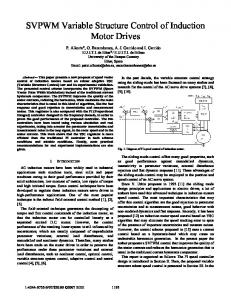
Fig. 1. Induction motor model in stationary reference frame (d-axis).

Fig. 3. Estimation block diagram.

Fig. 2.

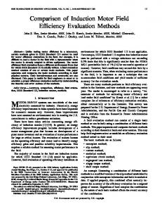
Stator resistance as a function of temperature.

core loss resistance models core losses. This resistance is estimated using a power approach and artificial neural networks. No additional hardware is necessary. The authors used the same power converter and DSP board that controls the motor in the industrial setting to generate the signals necessary to model the motor. Therefore, phenomenons related to operation (for example PWM effects) are captured in modeling.

Transient data was used to determine , , and . The data consisted in small disturbance at steady state by stepping the supply voltage amplitude by 10%. The tests encompass a wide variation of frequency, supply voltage, and load. The frequency was varied from 30 Hz to 80 Hz in steps of 10 Hz. The supply voltage was varied from 10% to 100% of the rated voltage value in steps of 10% for each frequency. The load was varied from no-load to maximum load in eight steps. A total of 290 data files were obtained. The estimation was performed using a constrained optimization method available in Matlab (“constr”). Fig. 3 shows the block diagram of the estimation procedure. The induction motor model can be expressed in state space form as

II. INDUCTION MOTOR MODEL Fig. 1 represents the induction motor model used in this research ( -axis, -axis are similar). As noted by [1], the model is identical (without any loss of information) to the more common -model in which the leakage inductance is separated in stator and rotor leakage. The core loss branch is added to account for both stator and rotor core losses.

(2) (3) where

III. PARAMETER ESTIMATION A. Estimation of The estimation of the stator resistance is based on a dc test. A small positive reference (that maintains the current below its rated value) is set between phases A–B and C–B using the power is calculated as converter. (1) To capture the effect of temperature on the stator resistance, before each test, the motor was run with a higher load. The stator resistance test was performed immediately after the motor stopped. The temperature of the stator winding was also measured. The temperature dependency of the stator resistance is shown in Fig. 2.

and The initial conditions for the model were established as (4) The error between model and measurements was calculated as (5)

B. Estimation of

,

, and

For this part of the estimation, the core loss resistance was neglected. However, since the core loss resistance is about 100–2000 times higher than the rotor resistance, the error , and is minimal. introduced in the estimation of ,

The constrained optimization function is used to minimize the error function by modifying the parameter vector (6)

26


The initial values of the fluxes are not normally included in the parameter vector since they can be calculated from the initial conditions of the currents at steady state. However, these currents are noise corrupted and their measurement error will propagate into the calculation of the initial values of the flux. Furthermore, since flux equations have a large time constant, the initial condition error would influence the flux observation over the entire transient measurement (the self-correction of an otherwise convergent flux observer [22] will not have the time to correct the initial condition error) and will yield erroneous parameter estimates. The authors observed that the parameter vector modification increased the rate of convergence of the algorithm. Constraints were imposed as 10% of the rated value for on , , and and the lower bound and 300% for the upper bound. For the constraints were imposed as 200 of the saturation value (0.5 Wb).

Fig. 4.

Sensitivity of error to parameters as a function of slip at 60 Hz.

TABLE I CORRELATION BETWEEN PARAMETERS AND OPERATING CONDITIONS

IV. SENSITIVITY ANALYSIS Since an output error estimation method is used, there is no theoretical guarantee that the parameters will converge to their actual values. Therefore, it is necessary to study the effect of each parameter on the total error. It is obvious that those parameters with little effect on the total error will be more prone to estimation errors than parameters that affect it more. At steady state, the squared error per period can be calculated as

The sensitivity of the squared error to a parameter expressed as

(7) can be

(8) For the proposed model, the steady state current (complex form) can be expressed as

V. PARAMETER MAPPING TO OPERATING CONDITIONS Up to this point, the parameters of the motor were estimated for various operating conditions. The purpose of this section is to find the relation of the parameters to the operating conditions in a form that allows for use in a control environment. However, in order to be able to define an operating condition or to relate (map) a parameter to a condition, a correlation analysis is necessary. This establishes the “strong” and “weak” dependencies of parameters to operating variables. The authors selected intuitively the variables for the correlation study as , , , and . It could be argued that temperature is also a factor in this mapping. However, since the only temperature measurement available was the stator temperature (and was used for stator resistance calculation) it was not used in this correlation study. The correlation between two variables (in this case one variand the other a operating condition variable is a parameter ) can be defined as able (10)

(9) and and are the module and phase angle of . The sensitivity analysis was conducted for a slip ranging from 0 to 10% (larger values of are unobtainable at steady state) and a frequency from 20 Hz to 100 Hz. The rated values of the parameters were used. Fig. 4 shows a comparison of sensitivity , and at 60 Hz. for , or is It can be seen that the sensitivity of the error to low at small slip. Large errors can be introduced at low slip since their effect on the error is small. A limit of 2% on the slip was estimates below this imposed on the slip values. The and value are discarded. For large values of the slip the sensitivity decreases to 0. estimates for slip values of the error to larger than 2% were discarded.

where , are the mean of and , respectively, and , are their standard deviations. Table I shows the results of the correlation. Mapping consists in expressing the parameters of the motor as analytical functions of the operating conditions. A. Magnetizing Inductance, A strong correlation was observed between and . clearly saturates with an increase in . A second order polynoto in the mial was used to represent the dependency of saturated region. (11) Fig. 5 shows a comparison between the polynominal and the results of the estimation.


Fig. 5.

L

Fig. 6.

L

as function of I .

as function of I .

B. Leakage Inductance, A strong correlation was also observed between and . saturates with an increase in . A linear approximation was used to . to represent the dependency of (12) Fig. 6 shows a comparison between the polynomial and the results of the estimation. C. Rotor Resistance, Previous research has shown that the rotor resistance varies as a function of two factors: slip frequency (through skin effect) and rotor temperature (unmeasurable). However, Table I shows and but also . The dependency is a correlation between shown in Fig. 7. The correlation is due to the fact that both slip frequency and temperature are proportional to . The authors correlation holds only if the motor runs observed that the for a few minutes at a certain operating condition, to allow for temperature to reach a steady state. would not determine a sudden A sudden variation in if slip frequency remains constant since temperachange in relation can ture does not change as fast. Therefore, the only be used at steady state. In order to establish the influence , a test similar to a locked rotor was of slip frequency on used. The difference consists was that the rotor was not mechanically locked, but the voltages were small enough that the rotor would not move. The frequency was varied between 5 Hz and 120 Hz (1 Hz increments in the 5–10 Hz region and 10 Hz increments for the rest). Prior to each series of tests, the motor was run under a loading condition (no-load, medium load, and full load) to assure heating of the rotor.

Fig. 7.

R

Fig. 8.

Rotor resistance as function of ! for different temperatures.

27

as function of I .

A temperature sensor was mounted on the stator. This sensor was used for an indication when temperature has reached a steady state (for each loading condition). Fig. 8 shows the estimation as a function of slip frequency (for results of the locked rotor, equal to stator frequency). Since rotor temperature measurements are hardly possible, a precise off-line mapping of rotor resistance to operating conditions is impossible. However, the linearity relation (within the range of interest) between rotor resistance and slip frequency calculation. An on-line observer was develcan be used for oped (see Appendix). The observer is based on the assumptions that the rotor temperature varies much slower than the other variables (current, speed, etc.) and that steady state operating conditions exist (e.g., the motor is not in continuous transient). The rotor resistance dependency to slip frequency and rotor temperature can be expressed as (13) is the influence of temperature (unknown). in which The coefficient (influence of slip frequency) was estimated off line from the locked rotor tests measurements. At each operating condition (steady state), the values of the rotor resistance and of the slip frequency are estimated with the observer. Then for each loading condition (temperature) (14) Assuming that temperature changes slowly, at each instant of time, knowing the slip frequency allows for the determination of rotor resistance. Each time a steady state condition is detected, is reevaluated and rotor resistance calculated as function of slip frequency. It can be argued that since rotor resistance is

28

Fig. 9.


Rotor power losses for no-load test.

Fig. 10.

estimated, there is no need in determining . This is true while the motor operates at steady state. However, for efficiency optimization it is important to predict the variation of rotor resistance prior to a new steady state condition. VI. CORE LOSS ESTIMATION The disparity in values of rotor resistance and core loss resistance makes the simultaneous estimation of both close to impossible using a constrained optimization method. That is because the core loss resistance has a much smaller effect on the model output than the rotor resistance (i.e., a smaller sensitivity). One should also note that since the slip is nonzero for the no-load is already known, could be theoretically calcutest and at steady-state. However, even for most precise lated from speed encoders, the error in calculating a slip approaching zero could translate in an order of magnitude of error when calcu. lating The authors used a power-based approach for calculating the core resistance. The procedure is shown in the following. A. Calculate Rotor Losses at Frequencies of Interest Use the no-load tests and calculate the rotor power losses for each data set (15) A plot of these losses is shown in Fig. 9 for various frequencies. The losses increase with both the frequency and the rotor flux. B. Calculate Friction and Windage Losses Since core losses are zero when flux is zero, the intersection of the power curves with the vertical axis determines the friction and windage losses for a specific frequency. To find the friction and windage losses for all frequencies, an ANN was used to map the rotor losses to frequency and flux. More details on using ANN for mapping can be found in [3]. The mathematical relationship between the input and output patterns can be described as (16) is a nonlinear neural network mapping to be estabwhere lished. The ANN used in this study consists of two processing elements in the input layer. A single processing element in the output layer corresponds to the losses being modeled. The number of elements in the hidden layer is arbitrarily chosen

Mapping of rotor losses using ANN.

depending on the complexity of the mapping to be learned. A hyperbolic tangent transfer function is used in all hidden layer elements, while all elements in the input layer and output layer have linear (1:1) transformations. The back-propagation algorithm is used to train the neural network such that the between actual network outputs and sum squared error corresponding desired outputs is minimized over all training patterns . of (16) in terms After estimating the nonlinear mapping is comof the neural network, the network output puted from the 2 1 input vector according to the following equation: (17) denotes the matrix of connecting weights from the hidden is the weight matrix from the layer to the output layer. and are used input-layer to the hidden-layer. Bias terms as connection weights from an input with a constant value of one. The training patterns for the neural network models are composed of the no-load test data. Each data set is a vector of , , and . The results of the mapping are shown in Fig. 10. Friction and windage losses can be calculated for ANN at zero flux. A deterministic approach could have been used for determining windage and friction losses. However, such an approach would have required the use of a dynamometer to isolate windage and friction losses (they are a part of the total rotor losses). Furthermore, since an ANN model for total rotor losses was already developed, calculating windage and friction losses was seamless. C. Calculate Core Losses Core losses for each frequency and flux can be determined by subtracting the friction and windage losses and from the rotor losses (resistive rotor losses can be neglected at small slip).

where

(18) (19)

D. Calculate Core Resistance For each data point, calculate the core loss resistance (see Fig. 1) as (20)


Fig. 11.

Rotor core loss as function of flux and frequency.

Fig. 12.

Experimental setup. TABLE II INDUCTION MOTOR PARAMETERS (RATED)

29

Fig. 13.

Measured and calculated input power.

Fig. 14.

Estimation validation for 30 Hz test.

intense. The ANN part could not be implemented online with the TMS320C31 (it would have required a considerable increase in the control loop that would make the overall control scheme worse than without it). The authors expect that with the continuous increase in processing power of DSPs this will not be a problem in the future. VIII. MODEL VALIDATION

Map the core loss resistance to flux and frequency using ANN. The procedure is similar to the rotor loss mapping. Fig. 11 presents the results of the mapping. VII. EXPERIMENTAL SETUP The experimental setup used in this research is shown in Fig. 12. The induction motor is 3 phase, 4 pole, 5 Hp, 1750 rpm 220 V squirrel cage. The rated parameters of the motor are shown in Table II. The load is a 5 Hp synchronous generator supplying a variable resistor box. A variable dc power supply controls the excitation of the synchronous generator. The power converter is rated at 400 V/30 A and can switch at 20 kHz. A dual processor (TMS320C31 Master and TMS320P14 Slave) DSP board is used both for control and data acquisition. In order to avoid aliasing, the measured voltage is passed through a low pass filter prior to being acquired. The synchronous generator can be controlled simultaneously with the motor using the DSP board. The control is realized through the excitation voltage. The PWM cycle is 240 s and the data acquisition sampling time is 60 s. These values were chosen to accommodate the control algorithm and analytical model computation. Except for the ANN part, the analytical model is not very computational

A. Steady State-Power Input In order to validate the model at steady state, the authors used tests encompassing the entire range of operation of the induction motor. The frequency of the motor was varied from 30 to 70 Hz. The supply voltage was varied from 10% to 100% of rated. For each voltage and frequency entry, the load was varied from zero to maximum value. For all data sets, input power was measured and compared to the input power calculated using measured voltage and speed and the model. Fig. 13 shows the results of the comparison. B. Dynamic The model was used to predict the transient performance. Each test consisted in a large voltage step (20%) applied while the motor was running at steady state. Tests were conducted at various frequencies and voltages and loads. Figs. 14–16 present examples of the results in terms of the synchronously rotating reference frame currents. A second type of test consisted in transient behavior when starting the motor. The start-up currents (measured and simulated) are shown in the Fig. 17 in synchronous reference frame. For comparison, the simulation where constant parameters (rated values) are used is shown in Fig. 18.

30


IX. CONCLUSION

Fig. 15.


Fig. 16.


A systematic procedure for induction motor modeling was developed in this paper. The model includes the effects of inductance saturation (both for magnetizing and leakage inductance) and the effects of the core losses. It is also shown that there is a variation of rotor resistance as a function of slip frequency. The leakage inductance, magnetizing inductance and rotor resistance are estimated from transient data information using a constrained optimization method. Sensitivity analysis is employed to show that error sensitivity to parameters varies as a function of slip. The analysis eliminates parameters with that yield low sensitivity. Analytical functions are used to map the parameters to operating conditions. Since rotor resistance depends on temperature and slip frequency and the former is not measurable, an on-line rotor resistance observer was developed. Core losses are estimated using a power approach. ANN are used to map the total rotor losses (iron losses, friction, and windage losses) to flux and frequency. The core losses are obtained by subtracting the rotor losses at zero flux (generated by the ANN) from the rotor loss surface. The model is validated using tests covering various operating conditions. Since efficiency optimization is sought with this model, the model is shown to correctly predict the power input of the motor. For dynamic validation, input voltage disturbance tests and start-from-zero tests were employed. The model correctly predicted both tests. APPENDIX ROTOR RESISTANCE OBSERVER The motor is operating at steady state. a) Determine the supply frequency from current zero crossing. , b) Calculate slip frequency and slip as: continue if slip is larger than 2%. c) Filter currents with digital filter similar to the hardware based filter for voltages (see Section VIII) to account for the delay in voltage signals. d) Transform the variables into – stationary reference frame and calculate the instantaneous values of and

Fig. 17.

Transient response for start-up from zero speed.

e) Calculate and assuming and , reference phasors: f) The voltage expression ( -axis) can be written as

where Initialize g) Recursively estimate

Fig. 18. Transient response for start-up from zero speed with rated fixed parameters.

Calculate

, using least squares

are .


Calculate rotor resistance

REFERENCES [1] G. R. Slemon, “Modeling of induction machines for electric drives,” IEEE Trans. Ind. Applicat., vol. 25, pp. 1126–1131, Nov./Dec. 1989. [2] N. R. Klaes, “Parameter identification of an induction machine with regard to dependencies on saturation,” IEEE Trans. Ind. Applicat., vol. 29, pp. 1135–1140, Nov./Dec. 1993. [3] S. I. Moon, A. Keyhani, and S. Pillutla, “Nonlinear neural-network modeling of an induction machine,” IEEE Trans. Contr. Syst. Technol., vol. 7, pp. 203–211, Mar. 1999. [4] J. A. de Kock, F. S. van der Merwe, and H. J. Vermeulen, “Induction motor parameter estimation through an output error technique,” IEEE Trans. Energy Conv., vol. 9, pp. 69–76, Mar. 1994. [5] A. M. N. Lima, C. B. Jacobina, and E. B. F. de Souza, “Nonlinear parameter estimation of steady-state induction machine models,” IEEE Trans. Ind. Electron., vol. 44, pp. 390–397, June 1997. [6] L. A. de Souza Ribeiro, C. B. Jacobina, and A. M. N. Lima, “Linear parameter estimation for induction machines considering the operating conditions,” IEEE Trans. Power Electron., vol. 14, pp. 62–73, Jan. 1999. [7] P. Pillay, R. Nolan, and T. Haque, “Application of genetic algorithms to motor parameter determination for transient torque calculations,” IEEE Trans. Ind. Applicat., vol. 33, pp. 1273–1282, Sept. 1997. [8] E. Mendes and A. Razek, “A simple model for core losses and magnetic saturation in induction machines adapted for direct stator flux orientation control,” in Proc. Fifth Int. Conf. Power Electron. Variable-Speed Drives, vol. 388, London, U.K., 1994, pp. 192–197. [9] S. Ansuj, F. Shokooh, and R. Schinzinger, “Parameter estimation for induction machines based on sensitivity analysis,” IEEE Trans. Ind. Applicat., vol. 25, pp. 1035–1040, Nov./Dec. 1989. [10] J. Stephan, M. Bodson, and J. Chiasson, “Real-time estimation of the parameters and fluxes of induction motors,” IEEE Trans. Ind. Applicat., vol. 30, pp. 746–759, May/June 1994. [11] X. Xu and D. W. Novotny, “Implementation of direct stator flux orientation control on a versatile DSP based system,” IEEE Trans. Ind. Applicat., vol. 27, pp. 694–700, July/Aug. 1991. [12] J. K. Seok, S. I. Moon, and S. K. Sul, “Induction machine parameter identification using PWM inverter at standstill,” IEEE Trans. Energy Conv., vol. 12, pp. 127–132, June 1997. [13] C. Wang, D. W. Novotny, and T. A. Lipo, “An automated rotor time constant measurement system for indirect field-oriented drives,” IEEE Trans. Ind. Applicat., vol. 24, pp. 151–159, Jan./Feb. 1988.

31

[14] Y. N. Lin and C. L. Chen, “Automatic IM parameter measurement under sensorless field-oriented control,” IEEE Trans. Ind. Electron., vol. 46, pp. 111–118, Jan./Feb. 1999. [15] S. K. Sul, “A novel technique of rotor resistance estimation considering variation of mutual inductance,” IEEE Trans. Ind. Applicat., vol. 25, pp. 578–587, July/Aug. 1989. [16] T. Noguchi, S. Kondo, and I. Takahashi, “Field-oriented control of an induction motor with robust on-line tuning of its parameters,” IEEE Trans. Ind. Applicat., vol. 33, pp. 35–42, Jan./Feb. 1997. [17] L. C. Zai, C. L. DeMarco, and T. A. Lipo, “An extended Kalman filter approach to rotor time constant measurement in PWM induction motor drives,” IEEE Trans. Ind. Applicat., vol. 28, pp. 96–104, Jan./Feb. 1992. [18] D. J. Atkinson, P. P. Acarnley, and J. W. Finch, “Observers for induction motor state and parameter estimation,” IEEE Trans. Ind. Applicat., vol. 27, pp. 1119–1127, Nov./Dec. 1991. [19] S. Wade, M. W. Dunnigan, and B. W. Williams, “New method of rotor resistance estimation for vector-controlled induction machines,” IEEE Trans. Ind. Electron., vol. 44, pp. 247–257, Apr. 1997. [20] K. Matsuse, T. Yoshizumi, S. Katsuta, and S. Taniguchi, “High response flux control of direct-field-oriented induction motor with high efficiency taking core loss into account,” IEEE Trans. Ind. Applicat., vol. 35, pp. 62–69, Jan./Feb. 1999. [21] B. Robyns, P. A. Sente, H. A. Buyse, and F. Labrique, “Influence of digital current control strategy on the sensitivity to electrical parameter uncertainties of induction motor indirect field-oriented control,” IEEE Trans. Power Electron., vol. 14, pp. 690–699, July 1999. [22] K. Akatsu and A. Kawamura, “Online rotor resistance estimation using the transient state under the speed sensorless control of induction motor,” IEEE Trans. Power Electron., vol. 15, pp. 553–560, May 2000. [23] S. J. Chapman, Electric Machinery Fundamentals, 2nd ed. New York: McGraw-Hill, 1991.

Amuliu Bogdan Proca (S’96) received the B.S. degree from Universitatea Politehnica Bucharest, Bucharest, Romania, and the M.S.E.E. and Ph.D. degrees from The Ohio State University (OSU), Columbus, in 1992, 1997, and 2001, respectively. His research interests are in the areas of permanent magnet synchronous machine modeling, parameter estimation, and design.

Ali Keyhani (S’72–M’76–SM’89–F’98) received the Ph.D. degree from Purdue University, West Lafayette, IN, in 1975. From 1967 to 1969, he worked for Hewlett-Packard Co., Palo Alto, CA, on the computer aided design of electronic transformers. Currently, he is a Professor of Electrical Engineering at The Ohio State University, Columbus. From 1970 to 1973, he worked for Columbus and Southern Ohio Electric Company on computer applications for power system engineering problems. In 1974, he joined TRW Controls and worked on the development of computer programs for energy control centers. From 1976 to 1980, he was a Professor of Electrical Engineering at Tehran Polytechnic University, Tehran, Iran. His research interests are in control and modeling, parameter estimation, failure detection of electric machines, transformers, and drive systems.