MODELING AND MITIGATING BEAM SQUINT IN MILLIMETER WAVE

MODELING AND MITIGATING BEAM SQUINT IN MILLIMETER WAVE WIRELESS COMMUNICATION

A Dissertation

Submitted to the Graduate School of the University of Notre Dame in Partial Fulfillment of the Requirements for the Degree of

Doctor of Philosophy

by Mingming Cai

J. Nicholas Laneman, Director

Graduate Program in Electrical Engineering Notre Dame, Indiana March 2018

c Copyright by

Mingming Cai 2018 All Rights Reserved

MODELING AND MITIGATING BEAM SQUINT IN MILLIMETER WAVE WIRELESS COMMUNICATION

Abstract by Mingming Cai There has been increasing demand for accessible radio spectrum with the rapid development of mobile wireless devices and applications. For example, a GHz of spectrum is needed for fifth-generation (5G) cellular communication, but the available spectrum below 6 GHz cannot meet such requirements. Fortunately, spectrum at higher frequencies, in particular, millimeter-wave (mmWave) bands, can be utilized through phased-array analog beamforming to provide access to large amounts of spectrum. However, the gain provided by a phased array is frequency dependent in the wideband system, an effect called beam squint. We examine the nature of beam squint and develop convenient models with either a uniform linear array (ULA) or a uniform planar array (UPA). Analysis shows that beam squint decreases channel capacity, and therefore, path selection should take beam squint into consideration. Current channel estimation algorithms assume no beam squint, and channel estimation error is increased by the beam squint, further decreasing the channel capacity. Three problems involving phased-array beamforming are studied to incorporate and compensate for beam squint. First, we show that carrier aggregation can be used to improve system throughput to a point. We study the optimal beam alignment to maximize channel capacity, and demonstrate that, with sufficient band separation, focusing on only one band outperforms carrier aggregation. Approximations are de-

Mingming Cai veloped for a system with two symmetric bands to determine the critical values of system parameters like band separation, and angle of arrival beyond which it is preferable not to aggregate. Second, beamforming codebooks are designed to compensate for one-sided beam squint by imposing a channel capacity constraint. Analysis and numerical examples suggest that a denser codebook is required compared to the case without beam squint, and the codebook size increases as bandwidth or the number of antennas in the array increases and diverges as either of these parameters exceeds certain limits. Third, to decouple the transmitter and receiver arrays with two-sided beam squint, and to extend conventional codebook design algorithms, codebooks with a minimum array gain constraint for all frequencies and angles of arrival or departure are also designed to compensate for the beam squint. Again, either the bandwidth or the number of antennas in the array is limited by the effects of beam squint if the other one is fixed.

To the memory of my mom and grandpa

ii

CONTENTS

FIGURES . . . . . . . . . . . . . . . . . . . . . . . . . . . . . . . . . . . . . .

vi

TABLES

. . . . . . . . . . . . . . . . . . . . . . . . . . . . . . . . . . . . . .

ix

ACKNOWLEDGMENTS . . . . . . . . . . . . . . . . . . . . . . . . . . . . .

x

SYMBOLS . . . . . . . . . . . . . . . . . . . . . . . . . . . . . . . . . . . . .

xi

CHAPTER 1: INTRODUCTION 1.1 Overview . . . . . . . . . 1.2 Contributions . . . . . . 1.3 Outline . . . . . . . . . .

. . . .

. . . .

. . . .

. . . .

. . . .

. . . .

. . . .

. . . .

. . . .

. . . .

. . . .

. . . .

. . . .

. . . .

. . . .

. . . .

. . . .

. . . .

1 1 4 5

CHAPTER 2: BACKGROUND . . . . . . . . . . . . . . 2.1 Architectures for MmWave Beamforming . . . . 2.1.1 Analog Beamforming . . . . . . . . . . . 2.1.2 Hybrid Beamforming . . . . . . . . . . . 2.1.3 Digital Beamforming . . . . . . . . . . . 2.1.4 Phase and Beam Quantization . . . . . . 2.2 Beam Squint . . . . . . . . . . . . . . . . . . . . 2.2.1 System Model of the Receiver Array . . 2.2.2 Beam Squint Reduction and Elimination 2.3 Channel Models . . . . . . . . . . . . . . . . . . 2.3.1 Passband Propagation Model . . . . . . 2.3.2 Passband Array Model . . . . . . . . . . 2.3.3 Passband Beamforming Model . . . . . . 2.3.4 Discrete-Time Equivalent Channel Model 2.4 Related Topics . . . . . . . . . . . . . . . . . . 2.4.1 Initial Access and Channel Estimation . 2.4.2 Carrier Aggregation . . . . . . . . . . . . 2.4.3 Beamforming Codebook Design . . . . . 2.5 Summary . . . . . . . . . . . . . . . . . . . . .

. . . . . . . . . . . . . . . . . . .

. . . . . . . . . . . . . . . . . . .

. . . . . . . . . . . . . . . . . . .

. . . . . . . . . . . . . . . . . . .

. . . . . . . . . . . . . . . . . . .

. . . . . . . . . . . . . . . . . . .

. . . . . . . . . . . . . . . . . . .

. . . . . . . . . . . . . . . . . . .

. . . . . . . . . . . . . . . . . . .

. . . . . . . . . . . . . . . . . . .

. . . . . . . . . . . . . . . . . . .

. . . . . . . . . . . . . . . . . . .

6 6 6 7 8 9 9 11 15 17 18 19 20 22 24 24 26 27 28

iii

. . . .

. . . .

. . . .

. . . .

. . . .

. . . .

. . . .

CHAPTER 3: MODELING OF BEAM SQUINT 3.1 ULA with Beam Squint . . . . . . . . . . 3.2 UPA with Beam Squint . . . . . . . . . . 3.3 Discrete-Time Equivalent Channel Model 3.4 Summary . . . . . . . . . . . . . . . . .

. . . . . . . . . with . . .

. . . . . . . . . . . . . . . . . . . . . . . . Beam Squint . . . . . . . .

. . . . .

. . . . .

. . . . .

. . . . .

. . . . .

29 29 34 36 38

CHAPTER 4: EFFECTS OF BEAM SQUINT 4.1 Effect on Channel Capacity . . . . . . 4.2 Effect on Path Selection . . . . . . . . 4.3 Effect on Channel Estimation . . . . . 4.3.1 Channel Estimation with MLE 4.3.2 Channel Estimation of ULA . . 4.4 Summary . . . . . . . . . . . . . . . .

. . . . . . .

. . . . . . .

. . . . . . .

. . . . . . .

. . . . . . .

. . . . . . .

. . . . . . .

. . . . . . .

40 40 49 53 54 55 59

CHAPTER 5: CARRIER AGGREGATION WITH BEAM SQUINT 5.1 System Setup . . . . . . . . . . . . . . . . . . . . . . . . . . 5.2 Carrier Aggregation with One-Sided Beam Squint . . . . . . 5.2.1 Numerical Optimization . . . . . . . . . . . . . . . . 5.2.2 Carrier Aggregation of Two Symmetric Bands . . . . 5.2.3 To Aggregate or Not to Aggregate . . . . . . . . . . . 5.2.3.1 Increasing Band Separation . . . . . . . . . 5.2.3.2 Approximating the Critical Band Separation 5.2.3.3 Approximating the Critical AoA . . . . . . 5.2.3.4 Criterion for Whether or Not to Aggregate . 5.2.3.5 Numerical Results . . . . . . . . . . . . . . 5.3 Carrier Aggregation with Two-Sided Beam Squint . . . . . . 5.3.1 Numerical Optimization . . . . . . . . . . . . . . . . 5.3.2 Carrier Aggregation of Two Symmetric Bands . . . . 5.3.3 To Aggregate or Not to Aggregate . . . . . . . . . . . 5.3.3.1 Increasing Band Separation . . . . . . . . . 5.3.3.2 Criterion for Whether or Not to Aggregate . 5.4 Summary . . . . . . . . . . . . . . . . . . . . . . . . . . . .

. . . . . . . . . . . . . . . . . .

. . . . . . . . . . . . . . . . . .

. . . . . . . . . . . . . . . . . .

. . . . . . . . . . . . . . . . . .

. . . . . . . . . . . . . . . . . .

62 62 64 65 66 68 68 70 72 73 75 78 81 82 83 83 88 89

CHAPTER 6: BEAMFORMING CODEBOOK WITH CHANNEL CAPACITY CONSTRAINT . . . . . . . . . . . . . . . . . . . . . . . . . . . . . . 6.1 Definition of a Beamforming Codebook . . . . . . . . . . . . . . . . . 6.2 Properties of the Smallest Codebook . . . . . . . . . . . . . . . . . . 6.3 Codebook Design . . . . . . . . . . . . . . . . . . . . . . . . . . . . . 6.3.1 Odd-Number Codebook . . . . . . . . . . . . . . . . . . . . . 6.3.2 Even-Number Codebook . . . . . . . . . . . . . . . . . . . . . 6.3.3 Codebook Design Algorithm . . . . . . . . . . . . . . . . . . . 6.4 Constraint of the Fractional Bandwidth b . . . . . . . . . . . . . . . . 6.5 Numerical Results . . . . . . . . . . . . . . . . . . . . . . . . . . . . .

91 91 93 93 94 95 96 96 98

iv

. . . . . . .

. . . . . . .

. . . . . . .

. . . . . . .

. . . . . . .

. . . . . . .

. . . . . . .

. . . . . . .

. . . . . . .

6.6

6.5.1 Improvement of Channel Capacity . . . . . . . . . . . . . . . 98 6.5.2 Codebook Size . . . . . . . . . . . . . . . . . . . . . . . . . . 99 Summary . . . . . . . . . . . . . . . . . . . . . . . . . . . . . . . . . 101

CHAPTER 7: BEAMFORMING CODEBOOK DESIGN WITH ARRAY GAIN CONSTRAINT . . . . . . . . . . . . . . . . . . . . . . . . . . . . . . . . . 7.1 Definition of a Beamforming Codebook with Array Gain Constraint . 7.2 Beamforming Codebook Design . . . . . . . . . . . . . . . . . . . . . 7.2.1 Codebook Design Given Codebook Size . . . . . . . . . . . . . 7.2.2 Determination of the Minimum Codebook Size . . . . . . . . . 7.3 Limitations on System Parameters . . . . . . . . . . . . . . . . . . . 7.3.1 Generalized Beam Edge ψd and Optimized Codebook Array Gain gd . . . . . . . . . . . . . . . . . . . . . . . . . . . . . . 7.3.2 Fractional Bandwidth b . . . . . . . . . . . . . . . . . . . . . . 7.3.3 Number of Antennas N . . . . . . . . . . . . . . . . . . . . . 7.4 Numerical Results . . . . . . . . . . . . . . . . . . . . . . . . . . . . . 7.4.1 Examples of Codebook Design . . . . . . . . . . . . . . . . . . 7.4.2 Limitations on the Generalized Beam Edge ψd and the Optimized Codebook Array Gain gd . . . . . . . . . . . . . . . . . 7.4.3 Limitations on the Fractional Bandwidth b . . . . . . . . . . . 7.4.4 Limitations on the Number of Antennas N . . . . . . . . . . . 7.4.5 Diminishing Returns of Increasing Number of Antennas N . . 7.5 Summary . . . . . . . . . . . . . . . . . . . . . . . . . . . . . . . . .

102 102 105 105 110 113 113 115 115 117 119 119 123 124 124 127

CHAPTER 8: CONCLUSIONS AND FUTURE WORK . . 8.1 Conclusions . . . . . . . . . . . . . . . . . . . . . . 8.2 Future Work . . . . . . . . . . . . . . . . . . . . . . 8.2.1 Carrier Aggregation . . . . . . . . . . . . . . 8.2.2 Beamforming Codebook Design . . . . . . . 8.2.3 Channel Estimation . . . . . . . . . . . . . . 8.2.4 Beamforming in Frequency Division Duplex

. . . . . . .

. . . . . . .

. . . . . . .

. . . . . . .

. . . . . . .

. . . . . . .

. . . . . . .

. . . . . . .

. . . . . . .

. . . . . . .

128 128 129 129 129 130 130

APPENDIX A: PROOFS . . . . A.1 Proof of Theorem 1 . . . A.2 Proof of Theorem 2 . . . A.2.1 Codebook Size M A.2.2 Codebook Size M A.3 Proof of Theorem 3 . . . A.4 Proof of Theorem 4 . . .

. . . . . . .

. . . . . . .

. . . . . . .

. . . . . . .

. . . . . . .

. . . . . . .

. . . . . . .

. . . . . . .

. . . . . . .

. . . . . . .

131 131 133 133 134 135 138

. . . . . . . . . . . . . . . is Odd . is Even . . . . . . . . . .

. . . . . . .

. . . . . . .

. . . . . . .

. . . . . . .

. . . . . . .

. . . . . . .

. . . . . . .

. . . . . . .

. . . . . . .

. . . . . . .

BIBLIOGRAPHY . . . . . . . . . . . . . . . . . . . . . . . . . . . . . . . . . 140

v

FIGURES

2.1

Analog beamforming architecture. . . . . . . . . . . . . . . . . . . . .

7

2.2

Hybrid beamforming architecture. . . . . . . . . . . . . . . . . . . . .

8

2.3

Digital beamforming architecture. . . . . . . . . . . . . . . . . . . . .

9

2.4

Structure of a uniform linear array (ULA) with analog beamforming using phase shifters. . . . . . . . . . . . . . . . . . . . . . . . . . . .

10

2.5

Example of an angle response for a ULA. . . . . . . . . . . . . . . . .

14

2.6

Example of fine beam angle responses for different frequencies in a wideband system for ULA. . . . . . . . . . . . . . . . . . . . . . . . .

15

2.7

Reduction of Beam Squint with the Phase Improvement Scheme [32].

16

2.8

Illustration of nested channel models. . . . . . . . . . . . . . . . . . .

17

3.1

Example of array gain for a fine beam. . . . . . . . . . . . . . . . . .

31

3.2

Structure of a uniform planar array (UPA) with analog beamforming using phase shifters. . . . . . . . . . . . . . . . . . . . . . . . . . . .

33

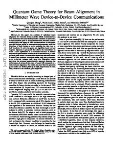
Examples of frequency-domain channel gains with and without beam squint for a ULA. . . . . . . . . . . . . . . . . . . . . . . . . . . . . .

39

Characteristics of |g (x)|2 from (3.7), its derivative, and its secondorder derivative within the main lobe. . . . . . . . . . . . . . . . . . .

44

4.2

Capacities with and without beam squint as a function of bandwidth.

47

4.3

The maximum and minimum relative capacity loss across the 3 dB beamwidth in a fine beam as a function of beam focus angle. . . . . .

48

Maximum relative capacity loss among all fine beams as a function of fractional bandwidth . . . . . . . . . . . . . . . . . . . . . . . . . . .

49

4.5

Example scenario of path selection with consideration of beam squint.

51

4.6

Channel capacities from path 1 and path 2 as function of AoA and AoD. 52

4.7

Example of MLE channel estimation with beam squint in the receiver.

56

4.8

MSE in a fine beam as a function of AoA for fixed beam focus angle.

58

4.9

The maximum MSE across 3 dB beamwidth in a fine beam as a function of beam focus angle. . . . . . . . . . . . . . . . . . . . . . . . . .

59

3.3 4.1

4.4

vi

4.10 The minimum MSE across 3 dB beamwidth in a fine beam as a function of beam focus angle. . . . . . . . . . . . . . . . . . . . . . . . . . . .

60

4.11 The maximum MSE across 3 dB beamwidth and beam focus angle range. 61 5.1 5.2

5.3

5.4 5.5 5.6 6.1 6.2 6.3

Example of aggregated channel capacities as functions of the band separation. . . . . . . . . . . . . . . . . . . . . . . . . . . . . . . . . .

69

Sub-optimal beam focus angles for two-band carrier aggregation obtained from numerical optimization and Approximation 1 as functions of band separation. . . . . . . . . . . . . . . . . . . . . . . . . . . . .

76

Maximum channel capacity for two-band carrier aggregation obtained from numerical optimization and Approximation 1 as functions of band separation. . . . . . . . . . . . . . . . . . . . . . . . . . . . . . . . . .

77

Critical band separations for two-band carrier aggregation of numerical optimization and Approximation 2 as functions of SNRr . . . . . . . .

79

Example of channel capacities for two-band carrier aggregation with two-sided beam squint as functions of the band separation. . . . . . .

86

Example of channel capacities for two-band carrier aggregation with two-sided beam squint as functions of the band separation. . . . . . .

87

Upper bound of the fractional bandwidth as a function of the number of antennas. . . . . . . . . . . . . . . . . . . . . . . . . . . . . . . . .

98

Capacity improvement ratio in a fine beam as a function of beam focus angle. . . . . . . . . . . . . . . . . . . . . . . . . . . . . . . . . . . . 100 Maximum capacity improvement ratio as a function of fractional bandwidth. . . . . . . . . . . . . . . . . . . . . . . . . . . . . . . . . . . . 100

6.4

Minimum codebook size in a ULA as a function of the number of antennas. . . . . . . . . . . . . . . . . . . . . . . . . . . . . . . . . . 101

7.1

Beamforming codebook design procedure with array gain constraint. . 105

7.2

Example of beamforming codebook design for the minimum codebook size subject to array gain constraint. . . . . . . . . . . . . . . . . . . 118

7.3

Generalized beam edge as a function of the codebook size for various fractional bandwidths. . . . . . . . . . . . . . . . . . . . . . . . . . . 120

7.4

Optimized codebook array gain as a function of the codebook size for various fractional bandwidths. . . . . . . . . . . . . . . . . . . . . . . 121

7.5

Optimized codebook array gain grows as codebook size increases . . . 122

7.6

Minimum codebook size as a function of fractional bandwidth. . . . . 123

7.7

Maximum relative approximation error as a function of the number of antennas. . . . . . . . . . . . . . . . . . . . . . . . . . . . . . . . . . 124

7.8

Minimum codebook size as a function of the number of antennas. . . 125

vii

7.9

Optimized codebook array gain as a function of the number of antennas.126

A.1 Relation between odd codebook size and even codebook size. . . . . . 139

viii

TABLES

1.1 7.1

COMPARISON BETWEEN SPECTRUM ACCESS BELOW 6 GHZ AND AT MMWAVE . . . . . . . . . . . . . . . . . . . . . . . . . . .

2

SUMMARY OF CODEBOOK PARAMETERS . . . . . . . . . . . . 111

ix

ACKNOWLEDGMENTS

First, I would like to express my sincere gratitude to my adviser and mentor, Dr. J. Nicholas Laneman. His support, encouragement, guidance, and patience have been indispensable part of this dissertation as well as my progress during my graduate study. Without his long-time words and deeds to help me improve my communication skills, I could not have won the People’s Choice Award in the Three Minute Thesis (3MT) competition of the graduate school in March 2017. I will always remember the whole night he stayed with me to improve algorithms and program for DARPA Spectrum Challenge. I would also like to thank Dr. Bertrand Hochwald. I have benefited significantly from his vision and experiences. He gave me many good suggestions not only on the radio design and implementation, but also on my career. My thanks also go to Ding Nie and Kang Gao. They are very smart and we have been working closely to make steady progress in our projects. I would like to thank Neil Dodson, as well. He substantially helped on the setup of lab environments. Zhanwei Sun, Nikolaus Kleber, Christine Landaw, Cindy Fuja, Jun Chen, Sahand Golnarian, Hamed Pezeshki, Abbas Termos, Chao Luo, Zhenhua Gong, Zhen Tong, Glenn Bradford, and Ebrahim MolavianJazi also provided me with good advice in my graduate study. I would like to thank them all. Last, but not least, I would like to express my gratitude to all my friends and my family for their support.

x

SYMBOLS

β θ ψ

phase shift angle of arrival or departure in uniform linear array (ULA), or azimuth angle in uniform planar array (UPA) virtual angle of θ

φ elevation angle ξ

ratio of subcarrier frequency to carrier frequency

λ wavelength σ 2 /2 Ω

spectral density of stationary white Gaussian noise angle of departure (AoD) or angle of arrival (AoA) in a UPA

ΩT

AoD in a UPA

ΩR

AoA in a UPA

Ψ

virtual AoD or AoA in a UPA

Θ

channel impulse response matrix for signal between Tx and Rx RF chains

a response vector of a ULA b fractional bandwidth c speed of light d distance between two adjacent antennas in a uniform array f

frequency

g

array gain of ULA

gT

transmitter array gain of ULA

gR

receiver array gain of ULA

h path gain

xi

r

received signal vector

s

transmitted signal vector

w

beamforming vector, i.e., weight vector of phase shifters

wT

transmitter beamforming vector, i.e., weight vector of phase shifters

wR

receiver beamforming vector, i.e., weight vector of phase shifters

z

Gaussian noise vector

B

bandwidth

C

channel capacity

C

codebook

D

relative capacity loss

G array gain of UPA GT

transmitter array gain of UPA

GR

receiver array gain of UPA

H

frequency-domain multipath channel matrix between Tx&Rx phase shifters

H

frequency-domain channel gain vector between Tx&Rx RF chains

I

capacity improvement

L

discrete delay spread

M

codebook size

N

number of antennas in a ULA

Na

number of antennas in a UPA

Nf

number of subcarriers in an OFDM symbol

Nh

number of antennas in horizontal direction of a UPA

Nl

number of paths in the channel model

Np

number of pilots in an OFDM symbol

Nv

number of antennas in vertical direction of a UPA

xii

CHAPTER 1 INTRODUCTION

1.1 Overview Applications of wireless technologies and the number of wireless devices have been growing significantly in the past decade. For example, the global mobile data traffic grew 63 percent in 2016, and it is expected to grow at a compound annual growth rate of 47 percent over the next five years [13]. There are increasing demands for radio spectrum to meet the requirements of higher data rates for an increasing number of mobile devices. As noted in a report from the President’s Council of Advisors on Science and Technology (PCAST), access to spectrum will be an increasingly important foundation for economic growth and technological leadership in the coming years [42]. However, the current process of long-term, static frequency allocation below 6 GHz cannot meet these demands for mobile spectrum. Two major directions are being explored for enhancing spectrum access, namely, reusing currently under-utilized spectrum through dynamic spectrum access (DSA), or spectrum sharing, and enabling access to spectrum at higher frequencies, e.g., millimeter-wave (mmWave) bands [7, 8, 18, 19, 38]. Although both directions require progress on interesting technical issues, this dissertation focuses on enabling spectrum access in mmWave bands based upon, on the one hand, its potential for wide bandwidths and less congested airwaves and, on the other hand, DSA’s ongoing regulatory and market uncertainties despite over a decade of significant research effort.

1

TABLE 1.1 COMPARISON BETWEEN SPECTRUM ACCESS BELOW 6 GHZ AND AT MMWAVE

Spectrum Below 6 GHz

mmWave

Spectrum Available

Hundreds of MHz

Tens of GHz

Signal Attenuation

Relatively small

Relatively large

Range / Coverage

Relatively large

Relatively small

Radio Cost

Relatively low

Relatively high

Regulatory Timelines

Relatively long

Relatively short

Table 1.1 summarizes the advantages and disadvantages of each of the two directions. There are several key features of mmWave bands that make them very attractive as the next frontier in wireless technology development. First, the mmWave band ranges from 30 GHz to 300 GHz, with spectrum opportunities on the order of tens of GHz wide. In a loose sense, the 20-30 GHz band is also considered part of the mmWave band, further increasing the amount of available spectrum. By contrast, the total amount of spectrum available for sharing below 6 GHz is limited, on the order of hundreds of MHz. Second, signals at mmWave frequencies experience higher path loss and atmospheric absorption, typically 20 dB or more attention, than those below 6 GHz. Therefore, mmWave systems often require higher antenna directionality and have comparatively smaller range or coverage than systems operating below 6 GHz. Third, relatively sparse deployments currently in mmWave bands leave much of the spectrum open to new entrants and simpler interference avoidance mechanisms, whereas the more congested spectrum below 6 GHz presents many technical

2

challenges for deployment of spectrum sharing such as spectrum sustainability and hidden nodes [23, 51, 59]. Fourth, commercially viable radio hardware for mmWave access is less mature than radio hardware operating below 6 GHz, and the device cost is usually higher. As development of device technologies for mmWave accelerates, the cost gap should close rapidly. A promising method to compensate for the higher attenuation in mmWave bands is beamforming [26]. To achieve high directional gain, either a large physical aperture or a phased-array antenna is employed [25, 27]. The energy from the aperture or multiple antennas is focused on one direction or a small set of directions. The cost of a large physical aperture is relatively high, especially in terms of installation and maintenance. Fortunately, the short wavelengths of mmWave frequencies in principle allows for integration of a large number of antennas into a small phased array, which would be suitable for application in commercial mobile devices. In mmWave beamforming, a phased array with a large number of antennas can compensate for the higher attenuation. In this dissertation, we consider practical implementations of mmWave analog beamforming with one radio frequency (RF) chain and a phased array employing phase shifters. Traditionally, in a communication system with analog beamforming, the set of phase shifter values in a phased array are designed at a specific frequency, usually the carrier frequency, but applied to all frequencies within the transmission bandwidth due to practical hardware constraints. Phase shifters are relatively good approximations to the ideal time shifters for narrowband transmission; however, this approximation breaks down for wideband transmission if the angle of arrival (AoA) or angle of departure (AoD) is far from the broadside because the required phase shifts are frequency-dependent. The net result is that beams for frequencies other than the carrier “squint” as a function of frequency in a wide signal bandwidth [34]. This phenomenon is called beam squint [21]. As we will see, beam squint translates

3

into array gains for a given AoA or AoD that vary with frequency, and becomes more pronounced if either the number of antennas in the array or the bandwidth increases.

1.2 Contributions This dissertation models beam squint, illustrates its effects on channel capacity and estimation, and develops approaches to mitigate it. Tradeoffs are provided among system parameters such as beam focus angle, bandwidth, number of antennas, and beamforming codebook size. The main contributions of the dissertation are summarized as follows. • Modeling beam squint. We model beam squint in a convenient way for a uniform linear array (ULA) and a uniform planar array (UPA). Throughout this dissertation, beam squint is incorporated into the discrete-time equivalent channel model whereas most current literature ignores beam squint in the channel model. • Effects of beam squint. The array gain varies over frequency due to beam squint, and this variation reduces channel capacity compared to the case without beam squint. Our analysis and numerical results show that the reduction in channel capacity increases with the number of antennas in the array, the bandwidth, or the beam focus angle. With beam squint affecting multiple paths for different AoD / AoA, a path with higher maximum array gain may actually provide a lower throughput. Therefore, we propose using channel capacity as the performance metric for path selection. Finally, current channel estimation algorithms do not consider beam squint, and we illustrate that beam squint increases channel estimation error. • Carrier aggregation with beam squint. In mmWave bands, multiple noncontiguous bands or carriers could be aggregated to provide more spectrum and therefore potentially higher channel capacity. We study carrier aggregation for mmWave considering beam squint, and we determine beam focus angles to maximize the total channel capacity. Specifically, we analyze the carrier aggregation problem for the case of two symmetric bands and provide design criteria based upon, among others, the band separation for determining if the beam should focus on the center of the two bands or if the beam should focus on only one of the bands. • Beamforming codebooks with channel capacity constraint. In switched beamforming, the transmitter and / or the receiver select a set of phase shifter values from pre-designed collection of such sets, the collection being called a 4

beamforming codebook. We introduce the problem of beamforming codebook design with beam squint subject to a constraint on the minimum channel capacity, and focus on the case of one-sided beam squint since this metric couples the transmitter and receiver design problems otherwise. The effects of beam squint increase the required codebook size, and substantially so as the number of antennas or the bandwidth increases. • Beamforming codebooks with array gain constraint. To be consistent with the majority of beamforming codebook research, we also design beamforming codebooks to compensate for beam squint subject to a minimum array gain for a desired angle range and for all frequencies in the wideband system. As we will see, beam squint with this design criterion fundamentally limits the bandwidth or the number of antennas of the array if the other one is fixed.

1.3 Outline An outline of the remainder of this dissertation is as follows. Chapter 2 provides a detailed background on mmWave beamforming. Specifically, current architectures for mmWave beamforming, channel models, channel estimation, and path selection techniques are summarized along with numerous references. We also qualitatively illustrate beam squint, and we summarize expensive hardware approaches to reduce or eliminate its effects. Chapter 3 develops models for beam squint for a ULA and a UPA, resulting in a baseband-equivalent models that incorporate beam squint. Chapter 4 illustrates the effects of beam squint on wireless communication systems, including effects on channel capacity, path selection, and channel estimation. Chapter 5 studies carrier aggregation with beam squint at mmWave. Chapter 6 develops a beamforming codebook design algorithm with channel capacity constraint. Chapter 7 designs beamforming codebooks with a minimum array gain constraint. Finally, Chapter 8 summarizes conclusions of the dissertation as well as directions for future research.

5

CHAPTER 2 BACKGROUND

In this chapter, we review existing work on mmWave beamforming, including architectures for mmWave beamforming, beam squint, channel models, initial access, channel estimation, carrier aggregation, and beamforming codebook design.

2.1 Architectures for MmWave Beamforming To compensate for high path loss and to achieve high directional gain, beamforming is employed in mmWave bands [25, 27]. Fortunately, the short wavelength of mmWave allows integrating a large number of antennas into a small phased array, which is suitable for the application of mobile devices. There are three basic architectures for mmWave beamforming, including analog beamforming, hybrid beamforming and digital beamforming.

2.1.1 Analog Beamforming Figure 2.1 illustrates the architecture of analog beamforming. Analog beamforming is implemented by a phased array with only RF chain driven by a digital-to-analog converter (DAC) in the transmitter or an analog-to-digital converter (ADC) in the receiver. A transmitter RF chain consists of frequency up converter, power amplifier and so on; a receiver RF chain consists of low-noise amplifier, frequency down converter and so on [5, 53]. The antenna weights in the phased array are constrained to be phase shifts that can be controlled digitally. The phases of the phase shifters are typically quantized 6

DAC

RF Chain

…

Baseband

Rx

…

Tx RF Chain

ADC

Baseband

Phase shifter

Analog Beamforming Figure 2.1. Analog beamforming architecture.

to limited resolution, and there is no ability to adjust the relative amplitudes of the signal fed into the antennas in the transmitter. The resulting transmit signal is constructive in some directions and destructive in other directions, forming a beam. The phases of the phase shifters can be dynamically adjusted based on specific strategies to steer the beam. Similar characteristics apply to the receiver.

2.1.2 Hybrid Beamforming The architecture of the hybrid beamforming is shown in Figure 2.2. On the transmitter side, there could be multiple data streams as the inputs to the Baseband Precoding block. Multiple DACs and RF chains are used and each of their outputs is combined to all or some of the antennas through phases shifters or switches in the RF Precoding Block [36]. On the receiver side, each signal from the antenna is connected to multiple phase shifters or switches, each for one RF chain and corresponding ADC. The signals from all or some of the antennas are combined to each RF chain separately. Similarly, there could be multiple data streams from the outputs of the Baseband Decoding Block. An alternative way to implement hybrid beamforming is using a large physical aperture [25, 27]. However, the cost of large physical aper-

7

DAC

DAC

RF Chain

RF Precoding

RF Combining

RF Chain

RF Chain

Tx

ADC

…

…

Baseband Precoding

RF Chain

Baseband Decoding

ADC

Rx Hybrid Beamforming

Figure 2.2. Hybrid beamforming architecture.

ture is relatively high, especially in terms of installation and maintenance. Hybrid beamforming can support multiple users and multiple data streams; however, the implementation complexity and cost are higher than those of analog beamforming.

2.1.3 Digital Beamforming The architecture of digital beamforming is illustrated in Figure 2.3 [58]. Each antenna is connected to its own RF chain and either a DAC or an ADC, making digital beamforming more flexible than analog beamforming and hybrid beamforming in terms of signal processing. However, there are three disadvantages of digital beamforming for mmWave. First, the array for mmWave needs to be packed into a small area, precluding a complete RF chain for each antenna. Second, the electronic components in each RF chain have large power consumption. Third, there could be Gigabits of data for each RF chain to process in a single second, and such high total data rate from all RF chains is a challenge for current baseband signal processing hardware. Analog beamforming is more appropriate for mobile mmWave applications be-

8

RF Chain

ADC

DAC

RF Chain

RF Chain

ADC

…

RF Chain

…

Baseband Precoding

DAC

DAC

RF Chain

RF Chain

ADC

DAC

RF Chain

RF Chain

ADC

Tx

Baseband Decoding

Rx Digital Beamforming

Figure 2.3. Digital beamforming architecture.

cause of its low cost and low complexity. Consequently, in this dissertation, we focus on analog beamforming.

2.1.4 Phase and Beam Quantization Based on whether or not the beam can be continuously adjusted in space, beamforming can be divided into two categories: continuous beamforming and switched beamforming. As implied by the name, beams in continuous beamforming can be adjusted continuously in space. In contrast, beams in switched beamforming can only be adjusted to focus on a finite set of angles. To cover a certain range of AoA/AoD in space, a beamforming codebook is usually used in switched beamforming [50, 55]. A beamforming codebook consists of multiple beams, with each beam determined by a set of beamforming phases. Each beam is a codeword of the codebook. The transmitter or receiver can only use one beam in its codebook at a time.

2.2 Beam Squint We consider a ULA with N identical and isotropic antennas as shown in Figure 2.4. 9

Signal ∆ ∆

∆

∆

1

2

Phase shifter

Broadside

∆

3

4

…

1

Splitter/Combiner RF Chain DAC/ADC

Figure 2.4. Structure of a uniform linear array (ULA) with analog beamforming using phase shifters. There are N antennas, labeled as 1, 2, 3, . . . , N . The distance between adjacent antennas is d, and θ denotes either the angle-of-arrival (AoA) for reception or the angle-of-departure (AoD) for transmission. The additional distance traveled by the electromagnetic wavefront from the first antenna to the nth antenna is denoted ∆dn .

10

The N antennas are labeled as 1, 2, 3, . . . , N . Each antenna is connected to a phase shifter. The distances between two adjacent antenna elements are the same and all denoted as d. For simplicity, we also assume the phases of the phase shifters are continuous without quantization. The AoA or AoD θ is the angle of the signal relative to the broadside of the array, increasing counterclockwise, and θ ∈ − π2 , π2 . This structure could represent the phased array of either a transmitter or a receiver, and their system analysis is similar. We focus on the receiver array for example.

2.2.1 System Model of the Receiver Array Suppose the signal arriving at the array is s (t) as shown in Figure 2.4. The signal received by the nth antenna is denoted as yn (t). Then the received signal vector y (t) before the phase shifters is

y (t) = [y1 (t) , y2 (t) , . . . , yN (t)]T ,

(2.1)

where superscript (·)T indicates transpose of a vector. As shown in Figure 2.4, the additional distance traveled by the signal from the first antenna to the nth antenna is denoted ∆dn , where

∆dn = (n − 1) d sin θ,

n = 1, 2, 3, . . . , N,

(2.2)

and ∆d1 = 0. Then y (t) can be denoted in terms of s (t) by T ∆d1 ∆d2 ∆dn ∆dN y (t) = s t − ,s t − ,...,s t − ,...,s t − c c c c T (n − 1) d sin θ (N − 1) d sin θ = s (t) , . . . , s t − ,...,s t − , (2.3) c c

11

where c is the speed of light. The frequency-domain received signal vector y (f, θ) is then h iT −1 −1 y (f, θ) = s (f ) , . . . , s (f ) ej2πc f (n−1)d sin θ , . . . , s (f ) ej2πc f (N −1)d sin θ h iT j2πc−1 f d sin θ j2πc−1 f (n−1)d sin θ j2πc−1 f (N −1)d sin θ = s (f ) 1, e ,...,e ,...,e , (2.4)

where y (f, θ) is a function of AoA θ, and θ ∈ − π2 , π2 . Define the ULA response vector as h iT −1 −1 −1 a (θ, f ) = 1, ej2πc f d sin θ , . . . , ej2πc f (n−1)d sin θ , . . . , ej2πc f (N −1)d sin θ ,

(2.5)

where θ ∈ − π2 , π2 [40]. a (f, θ) is frequency dependent. Then y (f, θ) = s (f ) a (θ, f ) .

(2.6)

The optimal combiner of the signal y (f, θ) should be a filter matched to a (f, θ) defined as

hM F (f, θ) = a∗ (θ, f ) h iT −j2πc−1 f d sin θ −j2πc−1 f (n−1)d sin θ −j2πc−1 f (N −1)d sin θ = 1, e ,...,e ,...,e , (2.7) where superscript (·)∗ denotes complex conjugate. The elements in the matched filter hM F (f, θ) are true-time-delay devices [33, 46]. However, the cost of true-timedelay devices is high, and there are also some implementation issues at mmWave band, which will be discussed in Section 2.2.2. In practice, phase shifters are used to approximate the optimal matched filter hM F (f, θ). A phase shifter is usually modeled as constant phase shift for all frequency within

12

its designed range [1, 21, 34]. The nth phase shifter is connected to the nth antenna with phase shift denoted by βn . Define the corresponding beamforming vector as T w = ejβ1 , . . . , ejβn , . . . , ejβN .

(2.8)

We note that w is frequency independent. Following [4], the array gain of the phased-array receiver with AoA θ and beamforming vector w is N 1 1 X j [2πc−1 f (n−1)d sin θ−βn ] g (w, θ, f ) = √ wH a (θ, f ) = √ e . N N n=1

(2.9)

where superscript (·)H denotes Hermitian transpose. Each beamforming vector w forms a beam in space. Among all the possible beams, we are interested in the ones that have the highest array gain, because the main purpose of beamforming at mmWave is to compensate for the high signal attenuation at mmWave bands. The set of phase shifters in the phased array is designed for a specific frequency, usually the carrier frequency, denoted as fc . Define the beam focus angle, denoted as θF , as the AoA/AoD with the highest array gain for the carrier frequency. To achieve the highest array gain for the carrier frequency and beam focus angle θF , the phase shifters should follow

βn (θF ) = 2πc−1 fc (n − 1) d sin θF , n = 1, 2, . . . , N.

(2.10)

Note that (2.10) corresponds to the matched filter (2.7) evaluated at θ = θF and f = fc . We call the beam with phase shifts described in (2.10) a fine beam, and we focus on the analysis of fine beams throughout this dissertation. Based on (2.9) and (2.10), the array gain for a signal with frequency f and AoA

13

Array Gain

4

2

0 -1.5

-1

-0.5

0

0.5

1

1.5

(rad)

Figure 2.5. Example of an angle response for a ULA with beam focus angle θF = 0. The number of antennas in the array N = 16. The antenna spacing is half of the wavelength corresponding to the carrier frequency fc = 73 GHz.

θ using beam focus angle θF is N 1 X j [2πc−1 (n−1)d(f sin θ−fc sin θF )] g (θF , θ, f ) = √ e . N n=1

(2.11)

Figure 2.5 shows an example of a fine beam angle response g(0, θ, fc ) at the carrier frequency for a ULA with 16 antennas. From the figure, the array only exhibits high gain for a small angle range. The fine beam acts as spatial filter so that the array gains for the other angles are relatively small. In general, the array response (2.11) varies with frequency across a wide bandwidth, which is the effect called beam squint [21, 34]. This results from the constant phase shift in the frequency domain of the fine beam corresponding to (2.10) instead of the linear phase shift in the ideal matched filter (2.7). Figure 2.6 illustrates beam squint by example, where the fine beam angle responses g(π/6, θ, fmin ), g(π/6, θ, fc ), and g(π/6, θ, fmax ) differ for signals with the same AoA/AoD θ. In particular, the

14

fmax

4

fc

fmin

2 0 -1

-0.5

0

0.5

1

Figure 2.6. Example of fine beam angle responses for different frequencies in a wideband system for ULA. The number of antennas in the array N = 16. The antenna spacing is half of the wavelength corresponding to the carrier frequency fc = 73 GHz, fmin = 65.7 GHz and fmax = 80.3 GHz.

array gains for θ = π/6 are smaller at both fmin and fmax compared to the gain at the carrier frequency fc .

2.2.2 Beam Squint Reduction and Elimination Several hardware-based approaches have been developed to reduce or eliminate beam squint. In [32], a phase improvement scheme shown in Figure 2.7 is proposed to reduce the effect of beam squint. In this scheme, banks of bandpass filters at mmWave are used to separate signals into smaller subbands; additional phase shifters are added to each subband to reduce the beam squint of each subband. Simulations show that the beam squint can be reduced. However, the signal components at the boundary of two subbands can be significantly distorted, and the bandpass filters increase cost.

To eliminate beam squint, true time-delay (TTD) devices can be applied [33, 46]. There are two basic methods to implement TTD: optical and electronic.

15

Filter

Filter

Filter

…

+

…

…

Transmitter RF chain

Filter

…

Tx

Filter

Filter

Filter

Filter

Rx +

Receiver RF chain

Phase shifter

Beam Squint Reduction with phase improvement scheme Figure 2.7. Reduction of Beam Squint with the Phase Improvement Scheme [32].

• In optical methods, RF signals are first modulated into optical signals, then the optical signals are delayed by long optical fibers to introduce time delay [35, 46], and finally the delayed optical signals are demodulated into RF signals again. To obtain different delays, multiple optical fibers are combined based on combination algorithms, such as binary fiber-optic delay line [20]. One disadvantage of optical TTD is its poor RF performance of the modulator and detector, such as 40 dB insertion loss [31]. Another issue is its large size and high cost, preventing mobile applications. • Electronic methods include coaxial cable, Micro-electro-mechanical Systems (MEMS), and monolithic microwave integrated circuits (MMICs) [33]. The weight of the TTD with coaxial cable is too large for mobile applications. MEMS TTD uses MEMS switches to combine the fabricated delay line on chip. The insertion loss is relatively small, such as 4 dB at 30 GHz [29]. MEMS is a promising technology for implementing TDD in mobile applications. However, it can fail with high power signals, a recent paper shows that a single MEMS TDD device has the size of tens of square millimeters, such as 4 mm × 9 mm [30], and the insertion loss for MMICs can be as much as 25 dB at 20 GHz [56]. In summary, the approaches outlined above are unappealing for mobile wireless communication due to combinations of high implementation cost, significant insertion loss, large size, or excessive power consumption. In this dissertation, we focus on system-level awareness of the effects of beam squint and developing algorithms to compensate for its negative effects. 16

Passband Beamforming Model Passband Array Model

Beamforming Vector 𝒘

𝑢

𝑥

𝑢 Array

𝑥

𝑠

𝑢

Frequency Up 𝑠 Converter

DAC

Passband Propagation Model

𝑣

𝑦

𝑣

𝑦 Array

…

𝑠

𝑥

𝑣

Passband Beamforming Model

Beamforming Vector 𝒘

𝑟

𝑦

𝑟

Frequency Down Converter

ADC

𝑟

Discrete-Time Equivalent Channel Model

Figure 2.8. Illustration of nested channel models.

2.3 Channel Models As shown in Figure 2.8, we consider four nested channel models for analog beamforming based on different encapsulated components. These channel models include three continuous-time models, namely, the passband propagation model, the passband array model, and the passband beamforming model, and one discrete-time equivalent channel model at baseband. Suppose there are NT and NR antennas in the transmitter and receiver, respectively. The AoD is denoted as θT , and the AoA is denoted as θR . Throughout this section, we consider a ULA for illustration. The models can be easily extended to a UPA.

17

2.3.1 Passband Propagation Model Propagation characteristics of mmWave signals are unique due to their relatively small wavelength compared to the objects in the environment [25]. Suppose there are Nl signal paths, labeled as 1, 2, . . . , Nl . The received signal of path l can be expressed as

vl (t) = gl ul (t − τl ) , l = 1, 2, . . . , Nl ,

(2.12)

where ul (t) is the sent signal of path l, gl is the channel gain of path l, and τl is the time delay of path l. Suppose the power of ul (t) is Pt , and the power of vl (t) is Pr . Based on Friis’ Law [44], if the signal is transmitted in free space, Pr = Pt Gt Gr

c 4πf dp

2 ,

(2.13)

where Gt is transmitter antenna gain, Gr is receiver antenna gain, c is the speed of light, dp is the distance between the transmitter and receiver antennas, and f is signal frequency. Therefore, the magnitude of gl can be expressed as √ |gl | =

Gt Gr c . 4πf dp

(2.14)

The Friis’ Law in dB scale can be expressed as 10 log10 (Pr ) [dB] = 10 log10 (Pt ) [dB] + 10 log10

Gt Gr c2 16π 2 f 2

− 20 log10 (dp ).

(2.15)

Friis’ Law indicates that the signal attenuation is proportional to the square of the frequency. Therefore, signals at mmWave experience much higher loss than signals below 6 GHz. This attenuation is one reason why beamforming is required at mmWave.

18

In practical environments, objects can attenuate, block or reflect signals. A significant amount of work has been performed to develop statistical models at mmWave for the distribution of path loss, especially on short-range links [48, 60]. From [25], the most commonly studied statistical model of path loss can be expressed as

P L (dp ) [dB] = α + 10γ log10 (dp ) + κ,

κ ∼ N 0, σ02 ,

(2.16)

where dp is the distance between the transmitter and receiver antennas, α is a constant, and γ is a log-normal random variable, and σ02 is variance of the path loss. Note that

20 log10 |gl | = −P L (dp ) [dB] .

(2.17)

Friis’ model (2.15) is a special case of (2.16) with γ = 2 almost surely.

2.3.2 Passband Array Model As shown in Figure 2.8, the passband array model describes the relation between the transmitted signal vector x (t) after phase shifters and the received signal vector y (t) before phase shifters, where

x (t) = [x1 (t) , x2 (t) , . . . , xNT (t)]T ,

(2.18)

y (t) = [y1 (t) , y2 (t) , . . . , yNR (t)]T .

(2.19)

From (2.5), the ULA response vectors for the transmitter and receiver are [40] h iT −1 −1 −1 aT (θT , f ) = 1, ej2πc f d sin θT , . . . , ej2πc f nd sin θT , . . . , ej2πc f (NT −1)d sin θT , (2.20) h iT −1 −1 −1 aR (θR , f ) = 1, ej2πc f d sin θR , . . . , ej2πc f nd sin θR , . . . , ej2πc f (NR −1)d sin θR , (2.21)

19

respectively, where θT , θR ∈ − π2 , π2 . The arrays are designed based on the carrier frequency. Typically, the antenna spacing is d = λc /2, where λc is the wavelength of the carrier frequency, i.e.,

λc =

c , fc

(2.22)

fc is the carrier frequency, and c is the speed of light. Doppler shift is the change of perceived signal frequency if the signal source moves towards or away from an observer. We assume the channel is slow fading so that the Doppler shifts of all paths are small and can be ignored [52]. Suppose path l has AoD θT,l , AoA θR,l , time delay τl , and complex path gain gl . According to [49], the frequency response of the passband array model is

H (f ) =

Nl X

−j2πτl f gl aR (θR,l , f ) aH , T (θT,l , f ) e

(2.23)

l=1

where (·)H denotes conjugate transpose. With this frequency-response definition, we have y(f ) = H(f )x(f ) + z (f ), which corresponds in the time domain to

y (t) =

Nl X

gl aR (θR,l ) aH T (θT,l ) x (t − τl ) + z (t) ,

(2.24)

l=1

where z(t) is a noise vector that captures the effects of thermal noise and other interference.

2.3.3 Passband Beamforming Model Phase shifters are part of the passband beamforming model. The effect of the phase shifters can be modeled by beamforming vector. The transmitter and receiver

20

beamforming vectors are T wT = ejβT,1 , . . . , ejβT,n , . . . , ejβT,NT , T wR = ejβR,1 , . . . , ejβR,n , . . . , ejβR,NR ,

(2.25) (2.26)

respectively, where βT,n is the phase of the nth phase shifter connected to the nth antenna in the transmitter array, and βR,n is the phase of nth phase shifter connected to the nth antenna in the receiver array. Again, the phase shifts βT,n , n = 1, 2, . . . , NT and βR,n , n = 1, 2, . . . , NR remain the same for all frequencies in the wideband of study due to hardware constraints [46]. Suppose sC (t) is the transmitted RF signal before the phased array and rC (t) is the received RF signal right after phased array as shown in Figure 2.8. Then

rC (f ) = HC (f ) sC (f ) + z (f ) ,

(2.27)

where z (f ) captures the effects of receiver thermal noise. From [4], the passband beamforming model can be expressed as 1 wR H H (f ) wT NR NT Nl X 1 −j2πτl f =√ gl wR H aR (θR,l , f ) aH , T (θT,l , f ) wT e NR NT l=1

HC (f ) = √

(2.28)

where the array response vectors aT (θT , f ) and aR (θR , f ) are, in general, frequencydependent. However, in current widely used channel models [25], the array response vectors are approximated to be constant across frequency. Specifically, the constant approximation often corresponds to evaluating the true array response only at the

21

carrier frequency fc . For this approximation, we define a0T (θT ) = aT (θT , fc ) h iT −1 −1 −1 = 1, ej2πc fc d sin θT , . . . , ej2πc fc nd sin θT , . . . , ej2πc fc (NT −1)d sin θT , (2.29) a0R (θR ) = aR (θR , fc ) h iT −1 −1 −1 = 1, ej2πc fc d sin θR , . . . , ej2πc fc nd sin θR , . . . , ej2πc fc (NR −1)d sin θR , (2.30)

so that the approximate passband beamforming model is

HC0

Nl X 1 H (f ) = √ gl wR H a0R (θR,l ) a0T (θT,l ) wT e−j2πτl f . NR NT l=1

(2.31)

We stress that, as we will see, beam squint becomes apparent in the true model (2.23), whereas it is hidden in the approximate model (2.31).

2.3.4 Discrete-Time Equivalent Channel Model To obtain a discrete-time equivalent channel model, we apply orthogonal frequencydivision multiplexing (OFDM) [12] with bandwidth B and Nf subcarriers. Label all the subcarriers as 0, 1, . . . , Nf − 1 with increasing frequency. The signals are down converted to baseband such that subcarrier Nf /2 is the DC tone. Suppose the baseband transmitted signal vector is s ∈ CNf ×1 , and the baseband received signal vector is r ∈ CNf ×1 . T s = s0 , s1 , . . . , sNf −1 , T r = r0 , r1 , . . . , rNf −1 .

22

(2.32) (2.33)

The discrete-time equivalent channel vector is denoted as

H = [H (0) , H (1) , . . . , H (Nf − 1)]T ,

(2.34)

where H ∈ CNf ×1 , and H (nf ) is the channel gain of subcarrier nf . The received noises for all subcarriers are independent and identically distributed (i.i.d) zero-mean Gaussian noise with variance σ 2 , and the noise vector is denoted as z. We have

r = H s + z,

(2.35)

where stands for Hadamard product, i.e., element-wise product. The beamforming vectors for subcarrier nf are iT h −1 −1 −1 aT (θT , nf ) = 1, ej2πc fnf d sin θT , . . . , ej2πc fnf nd sin θT , . . . , ej2πc fnf (NT −1)d sin θT , (2.36) iT h −1 −1 −1 aR (θR , nf ) = 1, ej2πc fnf d sin θR , . . . , ej2πc fnf nd sin θR , . . . , ej2πc fnf (NR −1)d sin θR , (2.37) where fnf is the frequency of subcarrier nf in the passband. Based on (2.28), the discrete-time equivalent channel model for subcarrier nf can be expressed as Nl n +N /2 X 1 −j2πχl f N f f gl wR H aR (θR,l , nf ) aH (θ , n ) w e H (nf ) = √ . T,l f T T NR NT l=1

(2.38)

where Nf is size of the OFDM symbol, χl is the delay of path l in the number of discrete-time samples. With the approximation of the array response vectors in (2.29) and (2.30), the commonly used approximate discrete-time equivalent channel model

23

is [25] Nl n +N /2 X 1 −j2πχl f N f H f gl wR H a0R (θR,l ) a0T (θT,l ) wT e . H (nf ) = √ NR NT l=1 0

(2.39)

H0 (nf ) in (2.39) can be reorganized as

0

H (nf ) = =

Nl X l=1 Nl X

gl

1 √ wR H a0R (θR,l ) NR

1 √ wT H a0T (θT,l ) NT

H

gl gR0 (wR , θR,l ) gT0 (wT , θT,l ) e

−j2πχl

nf +Nf /2 Nf

H e

−j2πχl

nf +Nf /2 Nf

,

(2.40)

l=1

where 1 gT0 (wT , θT,l ) = √ wT H a0T (θT,l ) , NT 1 gR0 (wR , θR,l ) = √ wR H a0R (θR,l ) . NR

(2.41) (2.42)

gT0 (wT , θT,l ) and gR0 (wR , θR,l ) are the transmitter and receiver array gains, respectively. Again, beam squint is not considered in gT0 (wT , θT,l ) and gR0 (wR , θR,l ).

2.4 Related Topics In this section, we review topics on initial access, channel estimation, carrier aggregation and beamforming codebook design, providing the background information for our discussion in Chapter 4 to Chapter 7.

2.4.1 Initial Access and Channel Estimation When the mmWave system starts up, the transmitter and receiver do not know on which directions their beams should focus. A process called initial access is required for the transmitter and receiver arrays to find the appropriate beam focus angles.

24

Selecting transmitter and receiver beams is equivalent to selecting a signal path, and ideally one of the strongest signal paths, for transmission. Usually, path gain (2.42) is used as the performance metric, because beam squint is typically ignored. There are four basic types of initial access schemes: exhaustive search, hierarchical search, compressive sensing and context information (CI)-based search [22]. In these initial access schemes, switched beamforming is assumed and therefore, a beamforming codebook is used. Continuous beamforming can be approximated with switched beamforming by increasing the number of beams in the codebook, i.e., codebook size. Details on the four initial access schemes are as follows. • Exhaustive Search is a brute-force search method in which all combinations of the transmitter and receiver beams are tested [28]. Suppose there are MT beams in the transmitter codebook and MR beams in the receiver codebook. There will be MT × MR tests. • Hierarchical Search consists of a a multi-stage scan of the angular space [16]. Each stage has a corresponding codebook. From the first stage to the last stage, the beamwidth of the beams in the codebook decreases. One beam in the codebook of previous stage covers the angle range of several beams in the next stage. In one stage, the best transmitter and receiver beams are found through exhaustive search. In the next stage, we only search through the beams that are covered by the beam in the previous stage. Usually, fine beams are used in the last stage. • Compressive Sensing (CS) techniques enable sparse channel recovery [24]. MmWave propagation tends to exhibit one line-of-sight (LOS) and a few nonLOS paths [43], and CS uses this sparse nature of the mmWave propagation to recover the channel with a small number of observations. • CI-Based Search is a location-assisted method [10]. Transmitter and / or receiver location information, such as GPS coordinates, is used to reduce the scope of the beam search. In exhaustive search and hierarchical search, there is a tradeoff between search time and average array gain of the codebook. The higher the average array gain for the codebook, the larger codebook size that is needed, and therefore, the longer the search time required.

25

A significant step in any of the initial access schemes is to estimate the channel to determine which beam is preferred, and for this, a channel estimation algorithm is required. Usually, wideband signal is used in mmWave beamforming, and therefore, the channel estimation algorithm must be compatible with the wideband signal. In mmWave system, OFDM could be used to provide higher spectral efficiency [45]. There are several pilot-aided channel estimation algorithms for OFDM, such as maximum likelihood estimator (MLE), minimum mean squared error (MMSE) estimator , and interpolation of pilots [17, 37]. Among the three, MMSE estimator has least channel estimation error, and interpolation provides the highest channel estimation error. MMSE estimator requires channel statistics, and MLE can be implemented in practice without channel statistics. We note that that current initial access schemes assume approximated channel model as shown in (2.31).

2.4.2 Carrier Aggregation In LTE, carrier aggregation is one of the technologies for increasing throughput by aggregating multiple component carriers or bands [45]. The bands could be contiguous or non-contiguous, providing flexibility in utilization of the spectrum [6, 54]. For mmWave bands, the bandwidth of each band could be much larger than the LTE band, such as 1 GHz to several GHz. Multiple non-contiguous bands could also be aggregated to further increase channel capacity [9]. To the best of our knowledge, current study of carrier aggregation in mmWave beamforming does not consider beam squint. However, beam squint causes array gain’s variation over frequency, making carrier aggregation in mmWave bands different from that at the microwave bands. Therefore, carrier aggregation in mmWave bands with beam squint should be explored to determine its application values.

26

2.4.3 Beamforming Codebook Design Beamforming has space selectivity, that is, the array gain is high around the beam focus angle, but small in other angle range. In switched beamforming, a codebook consists of multiple beam, and each beam is a codeword. Again, there is a tradeoff between the average array gain and the time or system overhedd to find the optimal beam within a codebook. Most current beamforming codebook designs assume that the beams in the codebook have the same angle response for all frequencies of study [3, 41, 57], and therefore, beam squint is ignored. These codebook designs focus on two directions, minimizing the effects of side lobes for reduced interference and maximizing the beamwidth while maintaining reasonable array gain. In practice, the array gains of different frequencies or subcarriers for a specific angle are not the same in the wideband system due to beam squint. Current study of the effect of beam squint on phased-array communication is merely on codebook design for linear arrays, and there are few publications discussing the effect of beam squint on codebook design [32, 55]. The authors in [55] mention that there is gain drop due to beam squint in their codebook design. The authors in [32] analyze the effect of beam squint on a codebook for IEEE 802.15.3c, and propose to reduce the effect of beam squint by applying extra phase shifts to different subbands using additional phase shifters and bandpass filters. Again, the added hardware increases the system complexity as well as cost and power consumption. It is therefore important to design beamforming codebooks considering beam squint to meet certain criteria without additional hardware.

27

2.5 Summary In this chapter, we summarized the architectures for analog beamforming, hybrid beamforming and digital beamforming, and motivated our focus on analog mmWave beamforming throughout this dissertation. A system model for a ULA employing analog beamforming was discussed, and we explained how beam squint results from using phase shifters instead of true-time-delay devices. Given that hardware-based methods to eliminate or reduce beam squint have higher complexity and cost, we proposed developing system designs and algorithms to work around the effects of beam squint. For this development in the remainder of the thesis, we summarized passband and baseband channel models that exhibit beam squint along with their simplification to ignore beam squint as is common in the literature. Fnally, we reviewed background information on initial access, channel estimation, carrier aggregation, and beamforming codebook design to set the stage for our discussion in Chapters 4 to 7.

28

CHAPTER 3 MODELING OF BEAM SQUINT

In this chapter, we model beam squint in both a uniform linear array (ULA) and a uniform planar arra (UPA), and we derive corresponding discrete-time equivalent channel models.

3.1 ULA with Beam Squint We consider a ULA with N identical and isotropic antennas as shown in Figure 2.4. AoA/AoD θ is the angle of the signal propagation path relative to the broadside of the array, increasing counterclockwise. The analysis of the effect of beam squint is the same for a transmitter or a receiver array. Without loss of generality, we focus on the case of a receive array. Traditionally, the beamforming vector w is designed for the carrier frequency. To achieve the highest array gain for a beam focus angle θF , the phase shifts in the beamforming vector w follow (2.10). The beam with phase shifts described in (2.10) is a fine beam, and we focus on the analysis of fine beams throughout the dissertation. For a wideband system, a subcarrier’s absolute frequency f can be expressed as

f = ξfc ,

(3.1)

where fc is the carrier frequency, and ξ is the ratio of the subcarrier frequency to the carrier frequency. Note that in this dissertation, the concept of subcarrier is not limited to an OFDM system. Suppose the baseband bandwidth of the signals of 29

interest is B. Then f ∈ fc − B2 , fc + B2 . Define the fractional bandwidth as b := B/fc ,

(3.2)

Then ξ ∈ [1 − b/2, 1 + b/2]. As a specific example, ξ varies from 0.983 to 1.017 in a system with 2.5 GHz bandwidth at 73 GHz carrier frequency. The array gain in (2.11) can be transformed into N 1 X j [2πc−1 fc (n−1)d(ξ sin θ−sin θF )] g (θF , θ, ξ) = √ e N n=1 N 1 X j [2πλ−1 c (n−1)d(ξ sin θ−sin θF )] =√ e , N n=1

(3.3)

where λc is wavelength of the carrier frequency. Let θ0 be the equivalent AoA for the subcarrier with coefficient ξ. Comparing (3.3) to (2.11), θ0 can be expressed as

θ0 = arcsin (ξ sin θ) .

(3.4)

The variation of beam patterns for different frequencies in the wideband system can therefore be interpreted as the variation of AoAs in the same angle response for different subcarriers. In other words, frequency variation and AoA variation due to beam squint are two sides of the same coin. Typically, the beamforming array is designed such that the antenna spacing satisfies

d=

λc . 2

(3.5)

Note that through this dissertation, d = λc /2 is the default value unless specifically stated. 30

4

fmin ( =1-b/2) fc ( =1)

2

0 -1

fmax ( =1+b/2)

-0.5

0

0.5

1

Figure 3.1. Example of g (x) from (3.7) for a fine beam with N = 16 antennas and antenna spacing d = λc /2. The curve in bold illustrates the array gain variations for different frequencies within the band.

From (3.3), N 1 X j[π(n−1)(ξ sin θ−sin θF )] e g (θF , θ, ξ) = √ N n=1 (N −1)π sin N2π (ξ sin θ − sin θF ) =√ ej 2 (ξ sin θ−sin θF ) , π N sin 2 (ξ sin θ − sin θF )

(3.6)

so that g (θF , θ, ξ) has linear phase of ξ sin θ − sin θF . If we define the single-argument function (N −1)πx sin N2πx g (x) = √ ej 2 , πx N sin 2

(3.7)

the array gain for frequency with ξ in (3.6) simplifies to g (ξ sin θ − sin θF ). Figure 3.1 illustrates an example plot of |g (x)|.

As can be seen, the side lobes

have much smaller gains, and our study focuses on the main lobe. The range of the main lobe in g (x) is x ∈ − N2 , N2 . The support of the main lobe in x is therefore N4 . In this dissertation, we focus on the magnitude (squared) of the array gain. Define 31

g −1 (y) , y ∈ R+ as the inverse function of |g (x)| for x ∈ 0, N2 , that is, given y as the magnitude of the array gain, g −1 (y) outputs the corresponding angle in the positive part of the main lobe. −g −1 (y) can be used for the angle in the negative part of the main lobe. Now let

ψ = sin θ

(3.8)

to convert the angle θ space to the ψ space. Correspondingly, the AoA becomes ψ = sin θ, the beam focus angle becomes ψF = sin θF , and ψF (w) = sin θF (w). The array gain for subcarrier ξ, AoA ψ, and beam focus angle ψF can then be expressed as (N −1)π sin N2π (ξψ − ψF ) g (ξψ − ψF ) = √ ej 2 (ξψ−ψF ) , π N sin 2 (ξψ − ψF )

(3.9)

where ψ, ψF ∈ [−1, 1]. The gain for subcarrier ξ at AoA ψ is equivalent to the gain for the carrier frequency at AoA ψ 0 = ξψ. The maximum array gain is

gm = max |g (ψ − ψF )| =

√ N

(3.10)

ψ∈[−1,1]

achieved by ψ = ψF . For simplicity, we study the effect of beam squint in ψ space. From (3.9) and Figure 3.7, the effect of beam squint increases as the AoA diverges from the beam focus angle, and it also tends to increase as the beam focus angle increases.

32

‫ݖ‬

… Signal

‫ݕ‬

߶

ܰ௩ antennas

ߠ ݀

Broadside

݀ Signal projection

‫ݔ‬

Figure 3.2. Structure of a uniform planar array (UPA) with analog beamforming using phase shifters. Each dot indicates one antenna, and each antenna is connected to one phase shifter. There are Na = Nh × Nv antennas, where Nh is the number of antennas in the horizontal direction and Nv is the number of antennas in the vertical direction. The distance between adjacent antennas is d. The AoA / AoD has two components: θ denotes the azimuth angle defined between the y axis and the signal’s projection on the x-y plane, and φ denotes the elevation angle defined between the signal and the x-y plane. Note that θ, φ ∈ [−π/2, π/2].

33

3.2 UPA with Beam Squint We consider a UPA as shown in Figure 3.2. The array is assumed to have Na = Nh × Nv antennas, where Nh is the number of antennas in the horizontal direction and Nv is the number of antennas in the vertical direction. One antenna can be located with coordinate (m, n), where m = 1, 2, . . . , Nv and n = 1, 2, . . . , Nh . θ and φ are used for the azimuth angle and elevation angle, respectively. The AoA/AoD consists of two components and is denoted

Ω = [θ, φ]T ,

(3.11)

Correspondingly, the AoD and AoA can be denoted as ΩT = [θT , φT ]T , and ΩR = [θR , φR ]T , respectively. The beam focus angle of the array is ΩF = [θF , φF ]T . The array gain of a UPA for a signal with wavelength λ, beam focus angle ΩF and AoA/AoD Ω is Nh Nv X X 1 −1 ej [2πλ ((n−1)d sin θ cos φ+(m−1)d sin φ)−βm,n (ΩF )] , G (ΩF , Ω) = √ Nv Nh m=1 n=1

(3.12)

where βm,n (ΩF ) is the phase of the phase shifter connected to antenna (m, n). Again, we consider fine beams designed for the carrier frequency with

βm,n (ΩF ) = 2πλ−1 c [(n − 1) d sin θF cos φF + (m − 1) d sin φF ] .

(3.13)

Similar to a ULA, the UPA array gain for subcarrier ξ can be expressed as Nh Nv X X −1 1 G (ΩF , Ω, ξ) = √ ej [2πλc ((n−1)dξ sin θ cos φ+(m−1)dξ sin φ)−βm,n (ΩF )] . (3.14) Nv Nh m=1 n=1

34

The UPA is designed with d = λc /2. From (3.13) and (3.14),

G (ΩF , Ω, ξ) Nh Nv X X 1 ej[π(n−1)(ξ sin θ cos φ−sin θF cos φF )+π(m−1)(ξ sin φ−sin φF )] =√ Nv Nh m=1 n=1 (Nh −1)π sin N2h π (ξ sin θ cos φ − sin θF ) ej 2 (ξ sin θ cos φ−sin θF cos φF ) =√ π Nh sin 2 (ξ sin θ cos φ − sin θF ) (Nv −1)π sin N2v π (ξ sin φ − sin φF ) ej 2 (ξ sin φ−sin φF ) . ·√ π Nv sin 2 (ξ sin φ − sin φF )

(3.15)

We denote virtual AoA/AoD as

Ψ = [ψ, ϕ]T ,

(3.16)

where the virtual azimuth angle and the virtual elevation angle are

ψ = sin θ cos φ,

(3.17)

ϕ = sin φ,

(3.18)

respectively. Since θ, φ ∈ [−π/2, π/2],

ψ 2 + ϕ2 = sin2 θ cos2 φ + sin2 φ ≤ cos2 φ + sin2 φ ≤ 1.

(3.19)

The feasible region of (ψ, ϕ) in two-dimensional space is a circle with radius 1. The phase of the phase shifter (m, n) for a fine beam with beam focus angle ΨF can then be expressed as

βm,n (ΨF ) = π [(n − 1) ψF + (m − 1) ϕF ] .

35

(3.20)

Furthermore, the array gain for beam focus angle ΨF , AoD/AoD Ψ and ξ is (Nh −1)π sin N2h π (ξψ − ψF ) ej 2 (ξψ−ψF ) G (ΨF , Ψ, ξ) = √ π Nh sin 2 (ξψ − ψF ) (Nv −1)π sin N2v π (ξϕ − ϕF ) ej 2 (ξϕ−ϕF ) ·√ π Nv sin 2 (ξϕ − ϕF ) = g (Nh ) (ξψ − ψF ) g (Nv ) (ξϕ − ϕF ) ,

(3.21)

where g (N ) (x) is the array gain of a ULA with N antennas in (3.7). Thus, the UPA’s array gain is the product of two ULA’s array gains with Nh and Nv antennas. The maximum array gain is therefore

Gm =

p Nh × Nv .

(3.22)

3.3 Discrete-Time Equivalent Channel Model with Beam Squint The discrete-time equivalent channel model with general beamforming vector has been derived in Section 2.3.4. In this section, we illustrate the discrete-time equivalent channel model based on the beam squint model of fine beams in Section 3.1. Although we only consider a ULA here, similar conclusions can be made for a UPA. As in Section 2.3.4, we consider an OFDM system with bandwidth B and Nf subcarriers. Index all the subcarriers as 0, 1, . . . , Nf − 1 with increasing frequency. Subcarrier Nf /2 is converted to DC tone. Suppose the discrete delay spread is L. We can assume that there are L paths, and that some of them may have zero channel gain, and we label the paths as l = 0, 1, . . . , L − 1. Suppose ξnf is the ratio of subcarrier frequency to the carrier frequency for subcarrier nf . Then

ξnf = 1 +

(2n − Nf + 1) b , 2Nf

36

n = 0, 1, . . . , Nf − 1,

(3.23)

so that Nf 1 X ξn = 1. Nf n=0 f

(3.24)

The transmitter and receiver array gains for subcarrier nf of path l can be denoted as gT ξnf ψT,l − ψT,F and gR ξnf ψR,l − ψR,F , respectively, where g (x) is defined in (3.9) and subscripts (·)T and (·)R denote transmitter and receiver, respectively. ψT,F and ψR,F are the beam focus angles for the transmitter and receiver, respectively. ψT,l is the AoD for path l, and ψR,l is the AoA for path l. Let hl,nf be the channel gain for path l and subcarrier nf . Then hl,nf = gl gR ξnf ψR,l − ψR,F gT ξnf ψT,l − ψT,F ,

(3.25)

where l = 0, 2, . . . , L − 1, nf = 0, 1, . . . , Nf − 1, and gl is the path gain between the transmitter and receiver arrays. Similar to (2.38), the channel gain between the transmitter and receiver RF chains for subcarrier nf is

H (nf ) = =

L−1 X l=0 L−1 X

f /2 −j2πl nf +N Nf gl gR ξnf ψR,l − ψR,F gT ξnf ψT,l − ψT,F e

−j2πl

hl,nf e

nf +Nf /2 Nf

, n = 0, 1, . . . , Nf − 1.

(3.26)

l=0

We denote the channel impulse response matrix for signal between transmitter and receiver RF chains as 

h0,Nf −1  h0,0 h0,1 . . .   h1,0 ... ... h1,Nf −1  Θ= .. ..  . . . . hl,n .   hL−1,0 . . . . . . hL−1,Nf −1

37

     ,   

(3.27)

where Θ is a L × Nf matrix. Then H = [H (0) , H (1) , . . . , H (Nf − 1)]T = Diag (QΘ) ,

(3.28)

where the operation Diag (·) generates a vector with the diagonal elements of a matrix, and Q is an Nf × L matrix with entries −j2πl

[Q]n,l = e

n+Nf /2 Nf

,

0 ≤ n ≤ Nf − 1,

0 ≤ l ≤ L − 1.

(3.29)

Figure 3.3 compares two examples of channel magnitude responses, both with and without beam squint. In the examples, the magnitude responses with beam squint have larger variation than those without beam squint.

3.4 Summary Array gain with beam squint was modeled for both a ULA and a UPA. The array gain variation over frequency for the same AoA/AoD is converted to the array gain variation over AoA/AoD for the carrier frequency. We also modeled the baseband-equivalent discrete-time channel with beam squint and demonstrated that its magnitude response varies more substantially over frequency with beam squint than without.

38

4 With Beam Squint Without Beam Squint

3.5

3

2.5 200

400

600

800

1000

1200

1400

1600

1800

2000

Subcarrier Index (a) 4.5 With Beam Squint Without Beam Squint

4 3.5 3 2.5 200

400

600

800

1000

1200

1400

1600

1800

2000

Subcarrier Index (b)

Figure 3.3. Examples of frequency-domain channel gains with and without beam squint for a ULA. There is no beam squint at in the transmitter, and noise is not considered. The number of antennas N = 16, the beam focus angle ψR,F = 0.9, AoA ψR,l = 0.94, fractional bandwidth b = 0.0342 (B = 2.5 GHz, fc = 73 GHz), and the number of subcarriers in an OFDM symbol Nf = 2048. (a) One path. (b) Two paths, path 0 and 15, with the same AoAs and with channel gain of path 15 being 10% that of path 0.

39

CHAPTER 4 EFFECTS OF BEAM SQUINT

Base on the beam squint model developed in Chapter 3, some effects of beam squint on wireless communication system are illustrated in this chapter, including effects on channel capacity, effects on path selection, and effects on channel estimation.

4.1 Effect on Channel Capacity This section illustrates the effects of beam squint on channel capacity for a ULA, with the understanding that there are similar effects in the case of a UPA. Although in general the effect of beam squint on capacity depends upon the AoD, the transmitter beam focus angle, the AoA, and the receiver beam focus angle, we consider for simplicity the case of no beam squint at the transmitter and study the beam squint of a single array at the receiver. Therefore, only the AoA and the receiver beam focus angle are examined here. Continuing from Section 3.3, we consider a complex channel and an OFDM system with bandwidth B and Nf subcarriers, labeled as 0, 1, . . . , Nf − 1. Equal power is allocated to all subcarriers at the transmitter, which is common if channel state information is not available at the transmitter. The total transmit power is denoted P , and the two-sided power spectral density of white Gaussian noise modeling receiver thermal noise is σ 2 /2. Due to poor scattering and significant attenuation of mmWave signals, the mmWave channel is sparse, that is, there is smaller number of significant signal paths compared

40

to that of microwave channels [2, 25, 43]. If fine beams are used at both the transmitter and receiver, most of the paths are filtered out by the two spatial filters. For simplicity here, we assume there is only one signal path, that is, L = 1 in the model of (3.26) with path gain g1 . The received power within bandwidth B at each receiver antenna before beamforming is denoted by

PR = P |gT g1 |2 ,

(4.1)

where gT is transmitter array gain. Viewing the OFDM system as a set of parallel Gaussian noise channels [15], the channel capacity is the sum of the capacities of each subchannel having bandwidth B/Nf . Incorporating beamforming with fine beams and accounting for beam squint in the receive array, the received power on subcarrier n with AoA ψ, beam focus angle ψF , and fractional bandwidth b is PR |g(ξn ψ − ψF )|2 , where g(·) is defined in (3.7), Similar to ξnf in (3.23), define

ξn = 1 +

(2n − Nf + 1) b , 2Nf

n = 0, 1, . . . , Nf − 1,

(4.2)

so that Nf 1 X ξn = 1. Nf n=0

(4.3)

Following Section 5.2.1 in [52], the channel capacity with beam squint at AoA ψ, beam focus angle ψF , and fractional bandwidth b is Nf −1

! 2 X B PR |g (ξn ψ − ψF )| CBS (ψF , ψ, b) = . log 1 + Nf n=0 Bσ 2

41

(4.4)

For comparison, the channel capacity without beam squint at AoA ψ and beam focus angle ψF is ! PR |g (ψ − ψF )|2 , CNBS (ψF , ψ) = B log 1 + Bσ 2

(4.5)

and we note that CNBS (ψF , ψ) is maximized if ψ = ψF . The proof is straightforward. All subcarriers in the case without beam squint achieve their largest array gain when ψ = ψF . For further discussion, we want to highlight some of the properties of the array gain function g(x) for x ∈ [−2/N, +2/N ], where g(·) is defined in (3.7). First, an important property to establish is the 3 dB point, i.e., the positive solution x3dB to the equation |g(x)|2 = |gm |2 /2,

x ∈ (0, +2/N ],

(4.6)

where gm is the maximum array gain of a ULA defined in (3.10). Numeric solution of (4.6) suggests that x3dB ≈ 2.78/(N π) [40]. For fixed fractional bandwidth b and beam focus angle ψF , we define the 3 dB beamwidth for all frequencies as the set of angles

R3dB (ψF , b) = ψ : |g(ξψ − ψF )|2 ≥ |gm |2 /2, ∀ξ ∈ [1 − b/2, 1 + b/2] ,

(4.7)

and with some manipulations, we obtain ψF + x3dB ψF − x3dB R3dB (ψF , b) = ψ : ≤ψ≤ , (1 − b/2) (1 + b/2)

42

(4.8)

and

|R3dB (ψF , b)| =

2x3dB − bψF . (1 − b2 /4)

(4.9)

Note that we focus on the 3dB beamwidth in the main lobe due to its large array gain. As we would expect, for the narrowband approximation b ≈ 0, |R3dB (ψF , 0)| = 2x3dB . Second, we characterize the concavity of |g(x)|2 . Figure 4.1 illustrates the squared magnitude |g (x)|2 , its derivative, and its second-order derivative as functions of x in the main lobe for N = 16. For the red portion of the curve in Figure 4.1(c), d2 |g(x)|2 ≤ 0, dx2 illustrating that |g (x)|2 is concave in that interval. The interval of concavity [−x∩ , +x∩ ] can be obtained by solving for the positive solution x∩ to the equation d2 |g(x)|2 = 0, x ∈ (0, +2/N ] . dx2

(4.10)

Numeric solution of (4.10) suggests that x∩ ≈ 2.61/(N π). For fixed fractional bandwidth b and beam focus angle ψF , we define the concavity beamwidth for all frequencies as the set of angles ( R∩ (ψF , b) =

) d2 ψ: |g(x)|2 ≤ 0, ∀ξ ∈ [1 − b/2, 1 + b/2] , dx2 x=(ξψ−ψF )

(4.11)

and with some manipulations, we obtain R∩ (ψF , b) =

ψ F − x∩ ψ F + x∩ ≤ψ≤ ψ: (1 − b/2) (1 + b/2)

43

,

(4.12)

20 10 0 -0.1

-0.05

0

0.05

0.1

0.05

0.1

0.05

0.1

(a) 200 0 -200 -0.1

-0.05

0 (b)

5000 0 -5000 -0.1

-0.05

0 (c)

Figure 4.1. Characteristics of |g (x)|2 from (3.7), its derivative, and its second-order derivative within the main lobe. The number of antennas in the ULA N = 16.

44

and

|R∩ (ψF , b)| =

2x∩ − bψF . (1 − b2 /4)

(4.13)

To study the relationship between CBS (ψF , ψ, b) and CNBS (ψF , ψ), we focus on angles ψ in the concavity width R∩ (ψF , b). Although this set of angles is smaller than the 3 dB beamwidth R3dB (ψF , b), which may seem more natural from a beamforming design perspective, the two are comparable. For example, in the narrowband approximation b ≈ 0,

|R∩ (ψF , 0)| / |R3dB (ψF , 0)| ≈ 93.9%

. Fact 1. For fixed fractional bandwidth b and beam focus angle ψF , if the AoA ψ ∈ R∩ (ψF , b) then

CBS (ψF , ψ, b) ≤ CNBS (ψF , ψ) ,

(4.14)

with equality if and only if ψ = 0. Proof. For fixed fractional bandwidth b and beam focus angle ψF , if the AoA ψ ∈ R∩ (ψF , b), we have Nf −1

! 2 X B PR |g (ξn ψ − ψF )| CBS (ψF , ψ, b) = log 1 + Nf n=0 Bσ 2   NP f −1 PR |g (ξn ψ − ψF )|2   a   n=0 ≤ Blog 1 +  Nf Bσ 2  

45

   b  ≤ Blog 1 +  

PR g

1 Nf

! 2  (ξn ψ − ψF )   n=0   2  Bσ 

NP f −1

PR |g (ψ − ψF )|2 = Blog 1 + Bσ 2

!

= CNBS (ψF , ψ) .

(4.15)

The inequalities (a) and (b) follow from Jensen’s Inequality [39], where. (a) is due to the concavity of the log function, and (b) is due to the concavity of |g (x)|2 for x ∈ [−x∩ , x∩ ]. The equality holds if and only if ψ = 0 for both (a) and (b), i.e., when there is no beam squint. We note that, outside R∩ (ψF , b), beam squint could actually increase the channel capacity. For example, if ψ = ±2/N , CNBS (ψF , ψ) = 0 and CBS (ψF , ψ, b) > 0. For ψ ∈ R3dB (ψF , b) but ψ ∈ / R∩ (ψF , b), the relation between CNBS (ψF , ψ) and CBS (ψF , ψ, b) must be examined on a case by case basis due to the concavity of log function and convexity of |g (x)|2 . We do not emphasize scenarios in which ψ ∈ / R3dB (ψF , b) in this dissertation, because the array gain is low. For a given receive power per transmit antenna PR , CNBS (ψF , ψ) increases with bandwidth B [15]. As B → ∞, CNBS (ψF , ψ) →

PR |g(ψ−ψF )|2 σ2

log2 e [15]. However, this

increasing trend does not apply to CBS (ψF , ψ, b). As B increases, CBS (ψF , ψ, b) has trends of first increasing and then decreasing. Figure 4.2 illustrates three examples. For small B, the effect of beam squint is limited, and CBS (ψF , ψ, b) increases due to the dominant effect of the growing bandwidth, similar to CNBS (ψF , ψ). As B further increases, the effect of beam squint dominates, and a larger portion of the subcarriers have smaller array gains. Some subcarriers may even fall outside the main lobe. Therefore, CBS (ψF , ψ, b) begins to decrease. Fact 1 suggests that beam squint decreases channel capacity for most practical 46

10 10

6

4

2

0 0

0.5

1

1.5

2 10

10

Figure 4.2. Capacity with beam squint CBS (ψF , ψ, b) and without beam squint CNBS (ψF , ψ, b) as a function of bandwidth for ψ = ψF = 0.9 with fixed PR /σ 2 = 2 × 109 Hz, and the number of subcarriers in an OFDM symbol Nf = 2048.

scenarios. To further illustrate the degree to which capacity decreases due to beam squint, we define the relative capacity loss as

D (ψF , ψ, b) =

CNBS (ψF , ψ) − CBS (ψF , ψ, b) . CNBS (ψF , ψ)

(4.16)

To study the effect of fractional bandwidth on channel capacity, 3 dB beamwidth without beam squint for ψF is defined as

R3dB (ψF ) = R3dB (ψF , b)|b=0 .

(4.17)

For fixed ψF and b, we defined the maximum relative capacity loss across the 3 dB beamwidth R3dB (ψF ) as

Dmax,ψ (ψF , b) =

max ψ∈R3dB (ψF )

47

D (ψF , ψ, b) ,

(4.18)

0.15

0.1

0.05

Dmax,

(

Dmin,

(

Dmax,

(

Dmin,

(

Dmax,

(

Dmin,

(

F F

,b) for N=64

F F

,b) for N=32

,b) for N=32

F F

,b) for N=64

,b) for N=16

,b) for N=16

0 0

0.2

0.4

0.6

0.8

1

Figure 4.3. Dmax,ψ (ψF , b) and Dmin,ψ (ψF , b) in a fine beam as a function of beam focus angle ψF . Here the number of subcarriers in an OFDM symbol Nf = 2048, fractional bandwidth b = 0.0342 (B = 2.5 GHz, fc = 73 GHz), PR and Bσ 2 = 0 dB.

Similarly, we define the minimum relative capacity loss across the 3 dB beamwidth R3dB (ψF ) as

Dmin,ψ (ψF , b) =

min ψ∈R3dB (ψF )

D (ψF , ψ, b) ,

(4.19)

For fixed b, the maximum relative capacity loss for all ψ ∈ R3dB (ψF ) and ψF ∈ [−1, 1] is defined as

Dmax,ψ,ψF (b) =

max Dmax,ψ (ψF , b) .

ψF ∈[−1,1]

(4.20)

Figure 4.3 shows examples of the maximum and minimum relative capacity loss across ψ ∈ R3dB (ψF ). Both Dmax,ψ (ψF , b) and Dmin,ψ (ψF , b) increase as N and |ψF | increase. Figure 4.4 illustrates that Dmax,ψ,ψF (b) increases as the fractional bandwith b increases, i.e., as the bandwidth increases for fixed carrier frequency.

48

0.2

N=4 N=8 N=16 N=32 N=64

0.15 0.1 0.05 0 0

0.01

0.02

0.03

0.04

Figure 4.4. Maximum relative capacity loss among all fine beams, Dmax,ψ,ψF (b), as a function of fractional bandwidth b. Here the number of PR subcarriers in an OFDM symbol Nf = 2048, and Bσ 2 = 0 dB.

In summary, the reduction in channel capacity increases with increases in any of the following: (a) the number of antennas in the array, N ; (b) the fractional bandwidth, b; (c) the magnitude of the beam focus angle, |ψF |.

4.2 Effect on Path Selection For environments in which there are multiple transmission paths between the transmitter and receiver, we might expect only one path to pass through the spatially selective fine beams on both sides. For the selected path, the transmitter and receiver will focus on the AoD and AoA of that path, respectively. This section demonstrates the need to consider path and beam selection jointly, and using channel capacity as the metric, when beam squint is significant. We consider again a ULA, with the understanding that analogous conclusions apply to UPA. 49

For concreteness, suppose the environment exhibits Nl transmission paths, labeled as l = 1, 2, . . . , Nl . Path l has AoD θT,l , AoA θR,l , and complex path gain gl . For simplicity, Doppler shift νl is ignored. Traditional path selection methods choose a path based on the largest end-toend channel gain incorporating the path gain as well as beamforming as in Design Criterion 1 [11]. Design Criterion 1 (Max Gain Path Selection). The selected path

l∗ = arg max |gl gR (ψR,l − ψR,F,l )gT (ψT,l − ψT,F,l )| ,

(4.21)

l∈{1,2,...,Nl }

where ψT,F,l and ψR,F,l are the transmitter and receiver beam focus angles designed for path l, respectively. If the AoD and AoA are known precisely, we can set ψT,F,l = ψT,l and ψR,F,l = ψR,l , so that the traditional path selection rule (4.21) becomes

l∗ = arg max |gl | ,

(4.22)

l∈{1,2,...,Nl }

corresponding to selecting the path with the largest gain. Neither of the path selection rules in (4.21) and (4.22) consider beam squint, but we have shown in the previous section that beam squint reduces channel capacity. Taking into account beam squint at both the transmitter and receiver, we conjecture that the path with the highest gain may not lead to the highest channel capacity. To motivate the conjecture, Figure 4.5 illustrates an example scenario with two paths, path 1 and path 2. The AoD and AoA of path 1 are both 0, and path 1 is shorter than path 2 but passes through a wall. Suppose the path gain of path 2 is slighter larger than that of path 1, i.e., |g2 | > |g1 |, due to the attenuation from the wall in path 1. If path selection is based on path gain only, path 2 would be selected. However, 50

Scatter

Path 2

Transmitter Array

Wall

Receiver Array

Path 1

Figure 4.5. Example scenario of path selection with consideration of beam squint.

based upon our results, we expect there to be beam squint and a reduction of channel capacity C2 on path 2, while there is no beam squint or reduction of channel capacity C1 on path 1. We expect that there will be scenarios in which C2 < C1 . With beam squint considered, the path selection criterion is stated in Design Criterion 2. Design Criterion 2 (Max Capacity Path Selection). For a scenario with Nl paths, consider beams focusing on path l, that is, ψT,F = ψT,l and ψR,F = ψR,l , resulting in channel capacity Cl , l = 1, 2, . . . , Nl . The selected path l∗ is l∗ = arg max Cl .

(4.23)

l∈{1,2,...,Nl }

We note that water filling [15] should be used to calculate channel capacity Cl , because AoA and AoD are known. 51

Channel Capacity (bits/sec)

1010

2.5

1 2 0.8 1.5

0.6

1

0.4

0.5

0.2

0

0 0

0.2

0.4

0.6

0.8

1

Figure 4.6. Channel capacities from path 1 and path 2 as function of AoA and AoD. ULAs are used in both the transmitter and receiver. ψR,F,l = ψR,l = ψT,F,l = ψT,l , and |g2 | = 1.1 |g1 |. The number of transmitter antennas NT = 64, and the number of receiver antennas NR = 16, the number of subcarriers in an OFDM symbol Nf = 2048, fractional bandwidth b = 0.0714 (B = 2 GHz and fc = 28 GHz, or B = 5.2 GHz and |g1 |2 fc = 73 GHz), and PBσ 2 = 0 dB.

Figure 4.6 continues exploring the example in Figure 4.5. It shows an example of the variations of C1 and C2 as AoA ψR,l and AoD ψT,l increase with ψR,l = ψT,l . The channel capacity is labeled on the left. C2 decreases significantly as AoA and AoD increase. If AoA and AoD are close to the broadside, i.e., ψT = ψR = 0, it is better to use path 2 for higher channel capacity due to g2 > g1 , which arrives at the same conclusion as using channel gain as the metric. However, as AoA and AoD increase, the channel capacity of path 2, C2 , decreases. To a certain value of AoA and AoD, it is better to use path 1 even if |g2 | = 1.1 |g1 | remains. C2 /C1 is also calculated with label on the right of the plot. C2 decreases significantly as AoA and AoD increase, further demonstrating the significance of using channel capacity for path selection.

52

4.3 Effect on Channel Estimation In the previous sections, channel gain is directly used for channel capacity calculation. However, in a practical system, channel gain is usually an unknown parameter. Often the receiver and sometimes the transmitter operate their modulation and coding scheme as well as beam patterns based upon estimates of the channel obtained, for example, from pilot or reference signals. Among the pilot-aided channel estimation algorithms for OFDM, MMSE estimator and MLE are widely used [17, 47]. In this dissertation, slow fading is assumed so that h is modeled as a fixed vector during the period of channel estimation and related transmissions. We use MLE to study the effect of beam squint on channel estimation. We will show beam squint significantly increases channel estimation errors of MLE, even without any noise. Again, we consider a ULA and an OFDM system with bandwidth B and Nf subcarriers, labeled 0, 1, . . . , Nf − 1, such that subcarrier Nf /2 is the DC tone. We expect the channel capacity would decrease as channel estimation error increases. Usually, the performance metric for channel estimation error is mean-square error (MSE) of the estimated channel between the Tx and Rx RF chains [37],  1 X ˆ 2 Γ0 = E  H (n) − H (n)  , Nf n=0 

Nf −1

(4.24)

ˆ (n) is the estimated channel gain of subcarrier where H (n) is the true channel, H n, and the expectation is over joint distribution. However, Γ0 varies with H (n). Therefore, the comparison with Γ0 is not fair for channel estimation errors of different array gains. To make fair comparison among different array sizes and AoA, we use

53

MSE of path gain between transmitter and receiver arrays, i.e, 



Nf −1

Γ (ψF , ψ, b) = E

X

|ˆ gl (ψF , ψ, b) − gl |2 ,

(4.25)

l=0

where gl is the path gain between arrays, gˆl is the estimated path gain between arrays

4.3.1 Channel Estimation with MLE In OFDM sysems, pilot or reference signals are usually used to assist in channel estimation. Suppose we have Np pilots uniformly located in the bandwidth B. Label the pilots as 0, 1, . . . , Np − 1, and let ip (n) ∈ {0, 1, . . . , Nf − 1}, n = 0, 1, . . . , Np − 1, denote the index of pilot n in the OFDM symbol. Denote the transmitted known pilot vector as sp , the received pilot vector as rp , and frequency-domain channel vector between the transmitter and receiver RF chains for pilots as Hp with beam squint embedded. Hp ∈ CNp ×1 and Hp = [H (ip (0)) H (ip (1)) . . . H (ip (Np − 1))]T ,

(4.26)

where ip (n) is the index of pilot n in the OFDM symbol. We also have T sp = sip (0) sip (1) . . . sip (Np −1) , T rp = rip (0) rip (1) . . . rip (Np −1) .

(4.27) (4.28)

The received pilot vector rp can be expressed as

rp = Hp sp + zp ,

(4.29)

where denotes Hadamard or element-wise product, and zp is independent and identically distributed Gaussian noise vector for the pilots. 54

From [37], the MLE of the channel impulse response in model (4.29) is

ˆ MLE = Qp H Qp h

−1

Qp H s∗p rp ,

(4.30)

where (·)H denotes conjugate transpose, (·)∗ denotes complex conjugate operation, and Qp is an Np × L matrix with entries −j2πl

[Qp ]n,l = e

ip (n)+Nf /2 Nf

, 0 ≤ n ≤ Np − 1, 0 ≤ l ≤ L − 1,

(4.31)

where L is discrete delay spread. The corresponding MLE of H is

ˆ MLE = A Qp H Qp ˆ MLE = Ah H

−1

Qp H s∗p rp ,

(4.32)

where A is a transform matrix with entries

[A]n,l = e

−j2πl

n+Nf /2 Nf

, 0 ≤ n ≤ Nf − 1, 0 ≤ l ≤ L − 1.

(4.33)

The MLE requires the invertibility of Qp H Qp , and the condition is met if and only if Qp is full rank and Np > L. In summary, the inputs of the MLE are sp , rp , and the indexes of the pilots. ˆ MLE . Figure 4.7 illustrates an example The output is the estimated channel vector H of MLE channel estimation. There is significant difference between the estimated channel and the actual channel, even without considering noise.

4.3.2 Channel Estimation of ULA In this section, we further show more numerical examples of the effect of beam squint on channel estimation when beam squint is not considered in MLE. A flat channel is considered. For simplicity, we assume there is no beam squint at the

55

5.5 H(n) ^ H(n)

5

jH(n)j

4.5 4

3.5 3 2.5 500

1000

1500

2000

Subcarrier Index

Figure 4.7. Example of MLE channel estimation with beam squint in the receiver. There is only one path and there is no beam squint in the transmitter. There is no additive noise. The number of antennas N = 16, beam focus angle ψF = 0.9, AoA ψ = 0.94, bandwidth B = 2.5 GHz, carrier frequency fc = 73 GHz, fractional bandwidth b = 0.0342, discrete delay spread L = 128, the number of subcarriers in an OFDM symbol Nf = 2048, and the number of pilots Np = 256.

transmitter and the power in the transmitter is equally assigned to each subcarrier. Therefore, the signal arrived at the receiver array is flat without beams squint while the receiver array has beam squint. From (4.25), 

Nf −1

Γ (ψF , ψ, b) = E|ˆ g0 (ψF , ψ, b) − g0 |2 +

X

 |ˆ gl (ψF , ψ, b)|2 

l=1

2  Nf −1 X ˆ H (n) H (n) 1   − =E , Nf n=0 g (ξn ψ − ψF ) g (ξn ψ − ψF ) 

(4.34)

where gl is the path gain between arrays, gˆl is the estimated path gain between arrays,

56

ˆ (n) is estimated frequency-domain channel gain , and equality ξn is defined in (4.2), H in (4.34) can be derived from Parseval’s theorem. The MSE is a function of ψF , ψ and b. For fixed beam focus angle ψF , the angle set within 3 dB beamwidth is R3dB (ψF ) as in (4.17). Figure 4.8 illustrates three examples of Γ (ψF , ψ, b) as a function of ψ for fixed beam focus angles ψF . There is no beam squint if ψ = 0. Within the 3 dB beamwidth, the MSEs on two sides tend to be higher than in the center. If ψF 6= 0, the smallest MSE in a beam is not located at ψF , but at a ψ with |ψ| < |ψF |. For certain ψF and b, the maximum MSE across ψ ∈ R3dB is defined as

Γmax,ψ (ψF , b) =

max ψ∈R3dB (ψF )

Γ (ψF , ψ, b) ,

(4.35)

and the minimum MSE across ψ ∈ R3dB is defined as

Γmin,ψ (ψF , b) =

min ψ∈R3dB (ψF )

Γ (ψF , ψ, b) .

(4.36)

Numerical examples of Γmax,ψ (ψF , b) and Γmin,ψ (ψF , b) are shown in Figure 4.9 and 4.10, respectively. Γmax,ψ (ψF , b) and Γmin,ψ (ψF , b) increase with ψF and N . If ψF > 0.9, the curve for N = 64 in Figure 4.9 is not smooth because the equivalent AoAs of some subcarriers are out of the main lobe. For certain b, the maximum MSE across ψ ∈ R3dB (ψF ) and ψF ∈ [−1, 1] is denoted as

Γmax,ψ,ψF (b) =

max Γmax,ψ (ψF , b) .

ψF ∈[−1,1]

(4.37)

Figure 4.11 shows Γmax,ψ,ψF (b) as a function of b. Within the main lobe, Γmax,ψ,ψF (b) increases as b increases, that is, Γmax,ψ,ψF (b) increases with the bandwidth for fixed carrier frequency. When b > 0.9, the curve for N = 64 is not smooth because the

57

10-5 10 5 0 -0.05

0

0.05

(a) 0.045 0.04 0.035 0.03 0.025 0.85

0.9

0.95

(b) 0.03 0.025 0.02 0.015 -0.95

-0.9

-0.85

(c)

Figure 4.8. MSE Γ (ψF , ψ, b) in a fine beam as a function of AoA ψ for fixed beam focus angle ψF . The dotted lines indicate Γmax,ψc (ψF , b) and Γmin,ψc (ψF , b), respectively. The number of antennas N = 16, fractional bandwidth b=0.0342 (B = 2.5 GHz, fc = 73 GHz), discrete delay spread L = 128, the number of subcarriers in an OFDM symbol Nf = 2048, and the number of pilots Np = 256. (a) Beam focus angle ψF = 0. (b) Beam focus angle ψF = 0.9. (c) Beam focus angle ψF = −0.9.

58

N=4 N=8 N=16 N=32 N=64

10 2

10 0

10 -2

10 -4 0

0.2

0.4

0.6

0.8

1

Figure 4.9. The maximum MSE across 3 dB beamwidth in a fine beam, Γmax,ψ (ψF , b), as a function of beam focus angle ψF . Fractional bandwidth b=0.0342 (B = 2.5 GHz, fc = 73 GHz), discrete delay spread L = 128, the number of subcarriers in an OFDM symbol Nf = 2048, and the number of pilots Np = 256.

equivalent AoAs of some subcarriers are out of the main lobe. To summarize these empirical results, the channel estimation error using MLE increases with increases in (a) the number of antennas in the array, N ; (b) the fractional bandwidth, b; (c) the magnitude of beam focus angle, |ψF |.

4.4 Summary We illustrated that beam squint reduces channel capacity, and the reduction of channel capacity increases with the number of antennas in the array, fractional bandwidth, and the magnitude of beam focus angle. In system with beam squint, channel capacity is also shown to be a better path selection criterion than channel gain. With 59

10 0 N=4 N=8 N=16 N=32 N=64

10 -1 10 -2 10 -3 10 -4 10 -5

0

0.2

0.4

0.6

0.8

1

Figure 4.10. The minimum MSE across 3 dB beamwidth in a fine beam, Γmin,ψ (ψF , b), as a function of beam focus angle ψF . Fractional bandwidth b=0.0342 (B = 2.5 GHz, fc = 73 GHz), discrete delay spread L = 128, the number of subcarriers in an OFDM symbol Nf = 2048, and the number of pilots Np = 256.

beam squint, the channel estimation error using MLE increases with the number of antennas in the array, fractional bandwidth, and the magnitude of beam focus angle.

60

N=4 N=8 N=16 N=32 N=64

10 4

10 2

10 0

10 -2

10 -4

10 -6

0

0.01

0.02

0.03

0.04

0.05

b

Figure 4.11. The maximum MSE across 3 dB beamwidth and beam focus angle range [−1, 1], Γmax,ψ,ψF (b), as a function of fractional bandwidth b. Discrete delay spread L = 128, the number of subcarriers in an OFDM symbol Nf = 2048, and the number of pilots Np = 256.

61

CHAPTER 5 CARRIER AGGREGATION WITH BEAM SQUINT

To the best of our knowledge, most existing works on beamforming only study a single band. In practice, the transmitter and receiver may access multiple noncontiguous bands to increase the throughput, i.e., carrier aggregation. Even if the bandwidth of each individual band is small, the aggregated channels from widely separated carriers can also introduce significant beam squint. In this chapter, we study carrier aggregation with beam squint for a ULA transmitter and a ULA receiver. Note that we consider only one RF chain for multiple bands considering the size and cost constraints of the user equipment (UE). Two beam squint scenarios are considered, carrier aggregation with one-sided beam squint and carrier aggregation with two-sided beam squint. Carrier aggregation with one-sided beam squint only considers beam squint in the receiver; carrier aggregation with two-sided beam squint assumes beam squint in both transmitter and receiver. We first study carrier aggregation with one-sided beam squint. Then the conclusion is applied to the study of carrier aggregation with two-sided beam squint.

5.1 System Setup The system setup in this section can be used for carrier aggragation with both one-sided and two-sided beam squint. We consider an OFDM system as in Chapter 3.3 to aggregate multiple noncontiguous bands. Suppose there are NB bands, labeled 1, 2, . . . , NB from the lowest 62

frequency to the highest frequency. The transmitter uses the NB bands to transmit data to the receiver. The bandwidths of the NB bands are B1 , B2 , . . . , BNB , respectively. The center frequencies of the NB bands are f1 , f2 , . . . , fNB , respectively, and

f1 < f2 < · · · < fNB .

(5.1)

To avoid overlap of any two bands, we must have

fi +

Bi+1 Bi ≤ fi+1 − , i = 1, 2, . . . , NB − 1. 2 2

(5.2)

We define the aggregate center frequency fa to be the center of all the bands, that is, f1 − fa =

B1 2

+ fNB +

BNB 2

2

.

(5.3)

Assume the ULA is designed based on the aggregate center frequency, that is, the distance between two adjacent antennas d = λa /2, where

λa =

c . fa

(5.4)

c is speed of light. Suppose there are Nf,i , i = 1, 2, ..., NB subcarriers in band i. The subcarriers of band i are indexed by n ∈ 0, 1, . . . , Nf,i − 1 with frequency increasing. The ratios of the subcarrier frequencies to the aggregate center frequency are defined as

ξi,n =

fi (2n − Nf,i + 1) Bi + , fa 2Nf,i fa

where i = 1, 2, ..., NB , and n = 0, 1, . . . , Nf,i − 1.

63

(5.5)

Assume the maximum transmission power across all bands is P . For simplicity, we assume that there is one dominant signal path with the same channel gain for all bands and that the remaining paths are filtered out by the transmitter and receiver array. Suppose the channel gain between the transmitter and receiver arrays is gp . The two-sided power spectral density of the stationary white Gaussian noise modeling thermal noise is σ 2 /2.

5.2 Carrier Aggregation with One-Sided Beam Squint For one-sided beam squint, beam squint can be on either the transmitter or the receiver side. In this dissertation, we consider carrier aggregation with beam squint on the receiver side, with the understanding that similar conclusions can be drawn with beam squint only at the transmitter. This scenario of no beam squint at the transmitter can be achieved if the AoD is 0◦ or true-time-delay devices are used at the transmitter. Suppose the transmitter array gain is gT . To maximize the channel capacity, water filling power allocation is used across bands. Based upon [52], the total channel capacity of all bands for the complex channel with beam squint at AoA ψ and beam focus angle ψF is ! NB 2 −1 ? X X P |g g g (ξ ψ − ψ )| B T p i,n F i i,n (N ) , log 1 + CWFB (ψF , ψ) = Bi 2 N σ f,i N n=0 i=1

(5.6)

f,i

? where subscript WF denotes water filling, and Pi,n is the power allocated to subcarrier

n of band i such that

? Pi,n

=

2 Bi ςi,n ν− Nf,i

+ , n = 0, 1, . . . , Nf,i − 1.

64

(5.7)

Here for i = 1, 2, . . . , NB and n = 0, 1, . . . , Nf,i − 1, 2 = ςi,n

σ2 , |gT gp g (ξi,n ψ − ψF )|2

(5.8)

and ν is chosen such that NB NX f,i −1 2 + X Bi ςi,n ν− = P, N f,i i=1 n=0

(5.9)

where (x)+ := max(x, 0). For a given AoA ψ, we would like to find the optimal beam focus angle ψF∗ to maximize the channel capacity in (5.6), that is, (N )

ψF∗ (ψ) = arg max CWFB (ψF , ψ) .

(5.10)

ψF

Note that the optimal beam focus angle could be beyond the (virtual) angle range of [−1, 1].

5.2.1 Numerical Optimization It turns out that the transmission power allocations vary with the beam focus angle ψF , increasing the difficulty to find the optimal beam focus angle. The optimal beam focus angle falls within the interval f1 fN B ψ, ψ , = fa fa

RBF

where subscript BF denotes beam focus angle. If ψF

fNB fa

ψ, the channel capacity cannot be maximized,

either.

65

Numerical optimization can be used to obtain an effective, though sub-optimal, beam focus angle. In the numerical optimization, the interval (5.11) is sampled into a finite set R0BF , defined as R0BF

(i − 1) (fNB − f1 ) f1 = ψF,i : ψF,i = ψ + ψ, i = 1, 2, . . . , NBF , (NBF − 1) fa fa

(5.12)

where there are NBF samples in R0BF . NBF is chosen to be an odd number such that the AoA ψ will be included in R0BF . The beam focus angle among R0BF that has the largest channel capacity is defined as (N )

∗ ψF,NO = arg max CWFB (ψF , ψ) .

(5.13)

ψF ∈R0BF

The subscript NO denotes numerical optimization. If there is more information on the band allocation, the information can be used to reduce the complexity of the numerical optimization. For example, if all the NB bands are symmetric with respect to the aggregate center frequency fa , i.e. Bi = BNB −i and fi + fNB −i = 2fa for i = 1, 2, . . . , NB , there should be two ψF∗ that are symmetric to ψ if ψF∗ 6= ψ, and only one ψF∗ if ψF∗ = ψ. Therefore, the range of the numerical optimization can be reduced to half the case without symmetry, and the number of samples required for the same resolution is reduced to

NBF +1 , 2

where NBF is odd.

5.2.2 Carrier Aggregation of Two Symmetric Bands In this section, we study carrier aggregation for the special case of two noncontiguous bands, band 1 and band 2. Both band 1 and band 2 have bandwidth B and their center frequencies are f1 and f2 , respectively. The system setup is similar to that in Section 5.1. f1 < f2 , and the two bands are located symmetrically with

66

respect to the aggregate center frequency fa , i.e.,

fa =

f1 + f2 . 2

(5.14)

The band separation or carrier separation, Bs , is the difference between f2 and f1 , i.e., Bs = f2 − f1 . To ensure there is no overlap between the two bands, we must have Bs ≥ B. Note that if Bs = B, the two bands can be treated as a single band. The ratio of subcarrier frequencies to aggregate center frequency for subcarrier n in band i, i = 1, 2 is

ξi,n = 1 + (−1)i

Bs (2n − Nf + 1) B + . 2fa 2Nf fa

(5.15)

Water filling power allocation is also employed to maximize the channel capacity. The total channel capacity of band 1 and band 2 with beam squint at AoA ψ and beam focus angle ψF is ! f −1 2 N 2 X X Pi,n |gT gp g (ξi,n ψ − ψF )| B (2) , log 1 + CWF (ψF , ψ, Bs ) = B 2 Nf i=1 n=0 σ N

(5.16)

f

where i is the band index. The water filling power allocation is the same as (5.7). (2)

CWF (ψF , ψ, Bs ) is a function of the band separation. The optimal beam focus angle becomes (2)

ψF∗ (ψ, Bs ) = arg max CWF (ψF , ψ, Bs ) .

(5.17)

ψF ∈RBF

Again, the optimal beam focus angle could be beyond the (virtual) angle range of [−1, 1].

67

5.2.3 To Aggregate or Not to Aggregate Beyond certain values of the system parameters, such as band separation, AoA, and SNR, it is preferable not to aggregate. We develop these results in this section.

5.2.3.1 Increasing Band Separation (2)

(2)

Figure 5.1 shows examples of CWF (ψ, ψ, Bs ) and CWF (ψf1 /fa , ψ, Bs ) as func(2)

tions of the band separation Bs . For CWF (ψ, ψ, Bs ), the beam focuses on the center (2)

of the two bands; for CWF (ψf1 /fa , ψ, Bs ) the beam focuses on the center of band (1)

1. The horizontal dotted line is CWF (ψ, ψ), in which only one channel with bandwidth B is used and the beam focuses on the center of that band. In general, (2)

(1)

CWF (ψf1 /fa , ψ, Bs ) ≥ CWF (ψ, ψ). Note that the fluctuation of channel capacity in Figure 5.1 occurs because one or two bands fall in a side lobe of the array response, which is beyond the scope of our study. As SNR decreases, the gap between (2)

(1)

CWF (ψf1 /fa , ψ, Bs ) and CWF (ψ, ψ) also decreases. If the band separation Bs is small, the two bands perform similarly to a single band. The maximum channel capacity is achieved if the beam focuses on the center of the two bands, that is, ψF∗ = ψ, because of symmetry and the concavity of |g (x)|2 for x ∈ [−x∩ , x∩ ]. This system is said to be in the Aggregation Regime. The (2)

corresponding channel capacity is CWF (ψ, ψ, Bs ). Fix ψF = ψ. As Bs increases, the two bands move away from the center of the main lobe of the array, the array gain decreases for both bands, and the channel capacity decreases. Eventually, as Bs continues to increase, the beam can be focused on one of the bands, i.e, ψF =

f1 ψ fa

or ψF =

f2 ψ, fa

resulting in higher channel capacity

as illustrated in Figure 5.1. The system is then said to be in the Disaggregation Regime. Although there could still be power allocated to the other band having low array gain, the marginal increase in channel capacity obtained from that band is small. (2)

The corresponding channel capacities for the two cases are CWF (ψf1 /fa , ψ, Bs ) = 68

1010


3 2.5 2 1.5 1 0.5 0 0

10

20

30

40

Band Separation (GHz)

(2)

Figure 5.1. Example of aggregated channel capacities CWF (ψ, ψ, Bs ) and (2) CWF (ψf1 /fa , ψ, Bs ) as functions of the band separation Bs . Critical band (1) separation Bs,c = 7.3 GHz. The horizontal dotted line is CWF (ψ, ψ), in which only one channel with bandwidth B is used and the beam focuses on (2) (2) the center of the band. If Bs < Bs,c , CWF (ψ, ψ, Bs ) > CWF (ψf1 /fa , ψ, Bs ); (2) (2) if Bs > Bs,c , CWF (ψ, ψ, Bs ) < CWF (ψf1 /fa , ψ, Bs ). The number of antennas in the array N = 32, AoA ψ = 0.8, channel bandwidth B = 2.5 GHz, and aggregate center frequency fa = 73 GHz. P |gT gp |2 = 5 dB, which is defined as SNRr in (5.24). Bσ 2

69

(2)

CWF (ψf2 /fa , ψ, Bs ), where the equality results from the assumed symmetry about the aggregate center frequency fa . (2)

Without loss of generality, we focus on CWF (ψf1 /fa , ψ, Bs ). Note that, in practice, band 1 may exhibit less signal attenuation than band 2 due to its lower frequency; however, the difference is not considered in this dissertation. If Bs increases (2)

(2)

to a certain point, CWF (ψ, ψ, Bs ) = CWF (ψf1 /fa , ψ, Bs ). The corresponding band separation is called the critical band separation denoted by Bs,c . If Bs > Bs,c , (2)

(2)

CWF (ψ, ψ, Bs ) < CWF (ψf1 /fa , ψ, Bs ). The natural beam focus angles in these two regimes are    ψ, ∗ ψF,sub (ψ, Bs ) =   f1 ψ or fa

Bs ≤ Bs,c , f2 ψ, fa

(5.18)

Bs > Bs,c ,

where the subscript sub denotes sub-potimal. The problem of determining an effective, though sub-optimal in general, beam focus angle then becomes identifying the critical band separation Bs,c . The critical band separation Bs,c can be obtained by numerically solving (2) CWF

f1 ψ , ψ, Bs,c fa

(2)

= CWF (ψ, ψ, Bs,c ) ,

(5.19)

for Bs,c , where

f1 = fa −

Bs,c . 2

(5.20)

5.2.3.2 Approximating the Critical Band Separation The critical band separation Bs,c can be obtained through numerical optimization if the number of samples is large. In this section, an approximation of the critical band separation is used.

70

Within each band, the beam squint may not be a dominant factor in channel capacity, especially if the bandwidth B is small. The array gain variation within band is smaller than that among bands. Therefore, we use the following approximation. Approximation 1. Beam squint is ignored within a band for both the Aggregation Regime and Disaggregation Regime, that is, different subcarriers within each band have the same array gain, and the channel capacity of each band can be approximated as the channel capacity without beam squint in that band. We note that beam squint is still considered across different bands. Water filling is used to allocate power to the bands to maximize the total channel capacity. (2)

CWF (ψF , ψ, Bs ) P ? |gT gp g (ψf1 /fa − ψF )|2 ≈ B log 1 + 1 Bσ 2

!

! P2? |gT gp g (ψf2 /fa − ψF )|2 + B log 1 + , Bσ 2 (5.21)

where P1? and P2? are power allocated to band 1 and band 2 according to water filling, respectively, similar to (5.7). If the beam focuses on the center of the two bands, i.e., ψF = ψ, equal power should be allocated to both bands due to symmetry. Therefore, the channel capacity can be approximated as P |gT gp g (ψf1 /fa − ψ)|2 (2) CWF (ψ, ψ, Bs ) ≈ 2B log 1 + 2Bσ 2  2  Bs P gT gp g ψ 2fa   = 2B log 1 + . 2Bσ 2

71

!

(5.22)

Combining (5.19), (5.21), and (5.22), 2  Bs,c P g g g ψ T p 2fa   2B log 1 +  2Bσ 2 

 2  √ 2  Bs,c P2 gT gp g ψ fa  P1 gT gp N    + B log 1 + = B log 1 +   . Bσ 2 Bσ 2 

(5.23)

Lemma 1. With Approximation 1, the critical band separation Bs,c is proportional to the aggregate center frequency fa and inversely proportional to the absolute value of AoA ψ. The proof is also straightforward. Bs,c only appears in (5.23) together with fa as Bs,c fa

and together with ψ as Bs,c ψ. Note that Lemma 1 needs not to apply to (5.19),

but does so approximately if the bandwidth B is small. Let P |gT gp |2 . SNRr = Bσ 2

(5.24)

SNRr measures the signal-to-noise ratio before the receiver array. Theorem 1. With Approximation 1, the critical band separation Bs,c monotonically increases as SNRr increases. The proof of Theorem 1 is in Appendix A.1. Theorem 1 shows that with lower SNR, the system is easier to enter Disaggregation Regime.

5.2.3.3 Approximating the Critical AoA If the band separation Bs , aggregate center frequency fa , and SNRr are fixed, the optimal beam focus angle depends on the AoA ψ. In this subsection, we also use Approximation 1. Similar to the critical band separation, there is also a positive 72

critical AoA defined as ψc . The channel capacities with various AoAs follow  (2) (2)   CWF (ψc , ψc , Bs ) > CWF (ψc f1 /fa , ψc , Bs ) , |ψ| < ψc ,    (2) (2) CWF (ψc , ψc , Bs ) = CWF (ψc f1 /fa , ψc , Bs ) , |ψ| = ψc ,      C (2) (ψc , ψc , Bs ) < C (2) (ψc f1 /fa , ψc , Bs ) , |ψ| > ψc . WF WF

(5.25)

If the absolute value of the AoA is smaller than ψc , it is better to focus on the center of the two bands; if the absolute value of the AoA is larger than ψc , it is better to focus on the center of one of the two bands. The sub-optimal beam focus angle should follow

∗ ψF,sub

   ψ, |ψ| ≤ ψc , =  fi ψ, |ψ| > ψ ,  c fa

(5.26)

where i = 1, 2. Note that the critical AoA ψc could be larger than 1. In this case, |ψ| is always smaller than ψc , and the beam focus angle should focuse on the center of the two bands, i.e., ψF = ψ, to maximize the total channel capacity. Similarly, with Approximation 1, the critical AoA ψc is inversely proportional to the band separation Bs , and proportional to the aggregate center frequency fa . With Approximation 1, the critical AoA ψ monotonically increases as SNRr increases.

5.2.3.4 Criterion for Whether or Not to Aggregate If the beam focuses on the center of one of the two bands, for example, band 1, the power allocated to band 2 is very small, and band 2 can be ignored in practice. Therefore, we use the following approximation. Approximation 2. In addition to Approximation 1, in the Disaggregation Regime, we further ignore the band with smaller array gain. In our case, band 2 is ignored and the total channel capacity can be approximated 73

as √ 2  P gT gp N   ≈ B log 1 + . Bσ 2 

(2)

CWF ψ

f1 , ψ, Bs fa

(5.27)

To solve for Bs,c , combine (5.19), (5.24) and (5.27) to obtain 0 2 2 Bs,c SNR r g ψ 2fa    = 1 + SNRr N . 1 + 2 

(5.28)

Therefore, s  √ Bs,c |ψ| 2 SNRr N + 1 − 2  = 2g −1  , fa SNRr

(5.29)

where g −1 (y) is defined as the inverse function of |g (x)| for x ∈ 0, N2 , and y ∈ R+ is the magnitude of the array gain, g −1 (y) outputs the corresponding angle in the positive part of the main lobe. −g −1 (y) can be used for the angle in the negative part of the main lobe. Fix band separation Bs , the critical AoA can also be obtained from (5.29). Based on (5.29), we have the following design criterion to determine whether to aggregate two bands or to use only one of them. Design Criterion 3. Given band separation Bs , AoA ψ, and SNRr , carrier aggregation should be applied if s  √ 2 SNRr N + 1 − 2  Bs |ψ| ≤ 2g −1  . fa SNRr

(5.30)

Otherwise, it is sensible to use only one band with the beam focused on the center of that band, i.e.,

f1 ψ fa

or

f2 ψ. fa

74

From (5.29), the critical band separation Bs,c is a function of SNRr . Define the function s √ 2 SNRr N + 1 − 2 . f (SNRr ) = SNRr

(5.31)

f (SNRr ) is a monotonically decreasing function of SNRr for SNRr > 0, and √ lim f (SNRr ) =

SNRr →0

lim

SNRr →∞

Since g

−1

N,

f (SNRr ) = 0.

(5.32) (5.33)

h √ i (y) is also a monotonically decreasing function of y for y ∈ 0, N ,

Bs,c ψ fa

monotonically increases as SNRr increases. Furthermore, √ Bs,c |ψ| −1 lim = 2g N = 0, SNRr →0 fa 4 Bs,c |ψ| = 2g −1 (0) = . lim SNRr →∞ fa N

(5.34) (5.35)

The critical AoA exhibits similar conclusions as (5.34) and (5.35) for a fixed Bs .

5.2.3.5 Numerical Results Figure 5.2 illustrates the estimated optimal beam focus angles with numerical optimization and Approximation 1. The plot indicates small differences between the two methods. These results suggest that the beam focus angle derived with Approximation 1 is reasonable in practice. Figure 5.3 shows the maximum channel capacities obtained from numerical optimization and Approximation 1. The channel capacities from the two methods exhibit small differences, showing the effectiveness of the approximations. Figure 5.4 compares the estimated critical band separations from numerical opti-

75

0.92 0.9 0.88 0.86 0.84 0.82 0.8 0

5

10

15

20

Figure 5.2. Sub-optimal beam focus angles for two-band carrier aggregation obtained from numerical optimization and Approximation 1 as functions of band separation Bs . NBF = 801, AoA ψ = 0.8, B = 2.5 GHz, and fa = 73 GHz.

76

1010

2.8 2.6 2.4 2.2 2 1.8 1.6 1.4 0

5

10

15

20

Figure 5.3. Maximum channel capacity for two-band carrier aggregation obtained from numerical optimization and Approximation 1 as functions of band separation Bs . NBF = 801, AoA ψ = 0.8, B = 2.5 GHz, and fa = 73 GHz.

77

mization and Approximation 2. With Approximation 2, the critical band separation (2)

is calculated based on (5.29). CWF (ψf1 /fa , ψ, Bs ) is obtained when the beam focuses on band 1, and no power is allocated to band 2 in the Disaggregation Regime. In Figure 5.4 (a), the Disaggregation Regime allows power to be allocated to band 2 for numerical optimization. The estimated critical band separations are very close if the SNRr is smaller than 5 dB, because power is not allocated to band 2 in numerical optimization due to water filling. As SNRr increases from 5 dB, there is an increasing gap between the two estimated critical band separations. The major reason is that power is allocated to band 2 in the Disaggregation Regime for numerical optimization and not by Approximation 2. To further verify this claim, we run another simulation to ensure that no power is allocated to band 2 in the Disaggregation Regime for numerical optimization. The results are illustrated in Figure 5.4 (b). The estimated critical band separations are very close, further demonstrating our claim. From Figure 5.4 (a), we can also observe that the critical band separation from numerical optimization is close to a constant if SNRr > 5 dB, which could be used to estimate the critical band separation for high SNRr .

5.3 Carrier Aggregation with Two-Sided Beam Squint In this section, we consider beam squint at both the transmitter and receiver ULAs. To maximize the channel capacity, water filling power allocation is also used across bands. Based on [52], the channel capacity of all bands with beam squint at AoD ψT , transmitter beam focus angle ψT,F , AoA ψR , and receiver beam focus angle ψR,F is

78

Critical Band Separation (GHz)

20

15

10

5

0 -10

-5

0

5

10

15

20

10

15

20

SNRr (dB)

(a) Critical Band Separation (GHz)

20

15

10

5

0 -10

-5

0

5

SNRr (dB)

(b)

Figure 5.4. Critical band separations for two-band carrier aggregation of numerical optimization and Approximation 2 as functions of SNRr . NBF = 801, AoA ψ = 0.8, B = 2.5 GHz, and fa = 73 GHz. In the Disaggregation Regime, the beam focuses on band 1. Power is (a) allowed and (b) not allowed on band 2 in numerical optimization..

79

(N )

CWFB (ψT,F , ψT , ψR,F , ψR ) = ! Nf,i −1 NB ? X |gT (ξi,n ψT − ψT,F )gp gR (ξi,n ψR − ψR,F )|2 Pi,n Bi X , log 1 + Bi Nf,i n=0 σ2 N i=1

(5.36)

f,i

? where Pi,n is the power allocated to subcarrier n of band i such that

? Pi,n

=

2 Bi ςi,n ν− Nf,i

+ , n = 0, 1, . . . , Nf,i − 1.

(5.37)

Here for i = 1, 2, . . . , NB and n = 0, 1, . . . , Nf,i − 1, 2 ςi,n =

σ2 , |gT (ξi,n ψT − ψT,F )gp gR (ξi,n ψR − ψR,F )|2

(5.38)

and ν is chosen such that NB NX f,i −1 2 + X Bi ςi,n ν− = P. Nf,i i=1 n=0

(5.39)

For fixed AoD ψT and AoA ψR , we would like to find the optimal beam focus T ∗ ∗ ψR,F to maximize the channel capacity in (5.36), that is, angle vector ψT,F

∗ ∗ ψT,F ψR,F

T

(N )

= arg max CWFB (ψT,F , ψT , ψR,F , ψR ) , T [ψT,F ψR,F ]

(5.40)

∗ ∗ ∗ ∗ where ψT,F and ψR,F are functions of ψT and ψR . Note that ψT,F and ψR,F could be

beyond the (virtual) angle range of [−1, 1].

80

5.3.1 Numerical Optimization The transmission power allocations are different for different beam focus angle ∗ T ∗ vector ψR,F ψR,F , increasing the difficulty to find the optimal beam focus angles. The optimal beam focus angles fall within the intervals fNB f1 ψT , ψT , RT,BF = fa fa fNB f1 ψR , ψR , RR,BF = fa fa

at the transmitter and receiver, respectively. If ψT,F < f1 ψ , fa R

or ψR,F >

fNB fa

(5.41) (5.42)

f1 ψ , fa T

ψT,F >

fNB fa

ψT , ψR,F
Bs,c , CWF,11 has the largest channel capacity. The number of antennas in the array NT = NR = 32, AoD and AoA ψT = ψR = 0.8, bandwidth B = 2.5 GHz, aggregate center frequency |gp |2 fa = 73 GHz, and signal-to-noise ratio PBσ 2 = 0 dB.

86

1010


5 4 3 2 1 0 0

10

20

30

40

Band Separation (GHz) (2)

(2)

(2)

Figure 5.6. Example of channel capacities CWF,bb , CWF,1b , CWF,bb , and (2)

CWF,11 for two-band carrier aggregation with two-sided beam squint as functions of the band separation Bs . The system critical band separation from numerical search is Bs,c = 7.8 GHz. The horizontal dotted line is (1) CWF (ψT , ψT , ψR , ψR ), in which only one channel with bandwidth B is used and the beam focuses on the center of the band. Generally, if Bs < Bs,c , (2) (2) CWF,bb has the largest channel capacity; if Bs > Bs,c , CWF,11 has the largest (2)

channel capacity. However, CWF,b1 is an outlier around Bs,c , because of side lobe. Therefore, the outlier is not considered. The number of antennas in the array NT = NR = 32, AoD ψT = 0.4, AoA ψR = 0.8, bandwidth B = 2.5 GHz, aggregate center frequency fa = 73 GHz, and signal-to-noise |gp |2 ratio PBσ 2 = 0 dB.

87

The natural beam focus angle vector in these two regimes is

∗ ψT,F,sub

  T T  [ψT ψR ] , ∗ ψR,F,sub = h iT h   f1 ψT f1 ψR or f2 ψT fa fa fa

Bs ≤ Bs,c f2 ψ fa R

iT

.

(5.49)

, Bs > Bs,c

The problem of determining an effective, though sub-optimal in general, beam focus angle vector then becomes identifying the critical band separation Bs,c . The (2)

(2)

critical band separation can be obtained by numerically solving CWF,bb = CWF,11 , i.e., (2)

(2)

CWF (ψT , ψT , ψR , ψR , Bs ) = CWF (ψT f1 /fa , ψT , ψR f1 /fa , ψR , Bs ) ,

with f1 = fa −

Bs,c , 2

(5.50)

or approximating it using (5.48).

5.3.3.2 Criterion for Whether or Not to Aggregate If the beams focus on the center of one of the bands, for example, band 1, the power allocated to the other band is very small and can essentially be ignored. Therefore, we apply Approximation 2, that is, in the Disaggregation Regime, we further ignore the band with smaller array gain in addition to Approximation 1. Define

SNR1 = SNR2 =

2 P gp gR ffa1 ψR − ψR Bσ 2 2 f1 P gp gT fa ψT − ψT Bσ 2

,

(5.51)

.

(5.52)

To obtain the critical band separation for the whole system, the critical band separations of each array is calculated separately assuming there is no beam squint in the other one. From Design Criterion 3 for one-sided beam squint, we have Design Criterion 4 for the two-sided beam squint to determine to aggregate or not to

88

aggregate. Design Criterion 4. Given band separation Bs , AoD ψT , AoA ψR , and SNR1 and SNR2 , we have two inequalities  √ 2 SNR1 NT + 1 − 2  Bs |ψT | ≤ 2g −1  , fa SNR1 s  √ 2 SNR2 NR + 1 − 2  Bs |ψR | ≤ 2g −1  , fa SNR2 s

(5.53)

(5.54)

where NT and NR are number of antennas in the transmitter array and receiver array, respectively. If both (5.53) and (5.54) are satisfied, carrier aggregation should be used with beam focus angles ψT and ψR at the transmitter and receiver, respectively. If either (5.53) or (5.54) is not satisfied, it is sensible to use only one band with the beam focus angles to be on the center of the used band, i.e., the transmitter and receiver, or

f2 ψ fa T

and

f2 ψ fa R

f1 ψ fa T

and

f1 ψ fa R

for

for the transmitter and receiver,

respectively. Either band 1 or 2 can be used. Usually, band 1 is preferred due to its lower frequency and smaller signal attenuation.

5.4 Summary We set up a one-sided carrier aggregation model for analog beamforming to maximize the overall channel capacity through the alignment of beam focus angle. Numerical optimization was used to obtain a sub-optimal beam focus angle because of the mathematical difficulty of solving for the optimal one. As a special case, we studied the carrier aggregation problem with two symmetric bands. In this scenario, a practical selection of the beam focus angle is either focusing on the center of two bands (Aggregation Regime) or one of the bands (Disaggregation Regime), depending 89

on the band separation, AoA, and SNR. Design criteria were developed to determine whether to use carrier aggregation or not and to approximate the critical parameter values beyond which we do not aggregate. We also studied two-sided carrier aggregation with beam squint. For arbitrary combinations of multiple bands, numerical optimization was also proposed to obtain sub-optimal beam focus angles for the transmitter and receiver. For the case of two symmetric bands, the two-sided carrier aggregation problem was treated as two onesided carrier aggregation problems. If either the transmitter or the receiver enters the Disaggregation Regime, the whole system enters Disaggregation Regime, according to the proposed design criteria.

90

CHAPTER 6 BEAMFORMING CODEBOOK WITH CHANNEL CAPACITY CONSTRAINT

This chapter treats the problem of designing a set of beams, called a beamforming codebook, to cover a given range of AoD or AoA. The beams (codewords) in the codebook should meet some minimum performance requirements, such as minimum channel capacity or minimum array gain. Current codebook design algorithms do not take beam squint into consideration, but as we have seen in Section 4.1, beam squint reduces channel capacity. Therefore, in this chapter, we design and analyze beamforming codebooks with consideration of beam squint subject to a constraint on the minimum channel capacity.

6.1 Definition of a Beamforming Codebook The system setup is the same as that for a ULA in Section 4.1. The (virtual) angle range to be covered by the codebook is denoted as RT , which we consider to be symmetric to the broadside,

RT = [−ψm , ψm ] ,

(6.1)

where 0 < ψm ≤ 1. The coverage of a fine beam w with beam focus angle ψF (w) and target rate Ct is the set of (virtual) angles

Rc (w, Ct , b) := {ψ ∈ RT : CBS (ψF (w), ψ, b) ≥ Ct } , 91

(6.2)

where CBS (ψF (w), ψ, b) is defined in (4.4). Selection of the capacity threshold Ct depends on the system design requirements. Generally, we can select the channel capacity without beam squint as a benchmark for Ct . For example, select (rgm )2 PR Ct (r) = B log 1 + Bσ 2

!

r 2 N PR = B log 1 + , Bσ 2

(6.3)

where 0 < r < 1, PR is the received power within bandwidth B at one antenna before beamforming defined in (4.1), and gm is the maximum array gain defined in (3.10). √ A reasonable choice is Ct,3dB = Ct 22 . Ct,3dB is the capacity without beam squint at the edge of 3 dB beamwidth, i.e., where the array gain is 3 dB below gm . The codebook is defined as the set of fine beams ( Ccap :=

w1 , w2 , . . . , wM :

M [

) Rc (wi , Ct , b) ⊇ [−ψm , ψm ] ,

(6.4)

i=1

where subscript cap denotes capacity. The ith beam in the codebook has weights wi and beam focus angle ψi,F = ψF (wi ). For convenience, we order the beam focus angles such that

−ψm ≤ ψ1,F < ψ2,F < · · · < ψM,F ≤ ψm .

(6.5)

The codebook size |Ccap | = M . Let Ωc be the set of all codebooks that meet the requirements of (6.4) for fixed values of N , b, Ct ,

PR , Bσ 2

and ψm . There is an infinite

number of codebooks in Ωc . Among them, we focus on the ones that achieve the minimum codebook size. The problem that needs to be solved is to find

Ccap,min = arg min Ccap ∈Ωc

92

|Ccap | .

(6.6)

6.2 Properties of the Smallest Codebook Define the left and right edges of the coverage of beam i as

ψi,l = min Rc (wi , Ct , b),

(6.7)

ψi,r = max Rc (wi , Ct , b),

(6.8)

respectively. The corresponding beamwidth is

∆ψi = ψi,r − ψi,l .

(6.9)

To achieve the minimum codebook size, there should be as little overlap as possible in the coverages among all the beams. One solution is

Rc (wi , Ct , b) ∩ Rc (wj , Ct , b) = ∅,

for i 6= j,

(6.10)

so that      

ψ1,l ≤ −ψm ψi+1,l = ψi,r ,

    

i = 1, 2, . . . , M − 1 .

(6.11)

ψM,r ≥ ψm

The codebook can therefore be designed by aligning the beams one by one.

6.3 Codebook Design There could be multiple codebook designs meeting the requirements in (6.11). Among them, we are more interested in the ones that are symmetric to the broadside. Before beam alignment, it is unknown whether the codebook with odd or even number of beams achieves the minimum codebook size. The codebook with odd number of

93

beams is called odd-number codebook, denoted as Co ; the codebook with even number of beams is called even-number codebook, denoted as Ce . Both the odd and even cases should be considered.

6.3.1 Odd-Number Codebook In the odd-number codebook Co , M is odd. Beam

(M +1) 2

is in the middle of all

beams, and its beam focus angle ψ M +1 ,F = 0. Given ψi,F , ψi,r can be derived by 2

solving

CBS (ψi,F , ψ, b) = Ct ,

(6.12)

where CBS (ψi,F , ψ, b) is defined in (4.4). Because of the symmetry of the main lobe with respect to the broadside, there should be two solutions. The larger one is ψi,r . We need to note that there could be no solution if the fractional bandwidth is larger than a threshold, which will be shown in Section 6.4. If there is no solution in solving for ψi,r , no codebook exists. Because there are no closed-form solutions to this equation, numerical methods must be applied. First, we find the beamwidth for Ct without beam squint, ∆ψCt , which is the difference between the two solutions of CNBS (ψF , ψ) = Ct , where CNBS (ψF , ψ) is defined in (4.5). All beams without beam squint have the same beamwidth in virtual angle. From Fact 1, ψi,r must satisfy

ψi,F ≤ ψi,r < ψi,F +

As ψ increases from ψi,F to ψi,F + Therefore, ψi,r

∆ψCt . 2

(6.13)

∆ψCt , 2

CBS (ψi,F , ψ, b) monotonically decreases. h ∆ψ can be found through binary search in the interval ψi,F , ψi,F + 2Ct

[14]. After the right edge of beam

(M +1) , 2

ψ M +1 ,r , is obtained, the left edge of beam 2

94

(M +3) 2

is

ψ M +3 ,l = ψ M +1 ,r . 2

(6.14)

2

The next step is to find ψ M +3 ,F given ψ M +3 ,l . Suppose ψi,l is known, ψi,F must follow 2

2

ψi,l ≤ ψi,F < ψi,l +

∆ψCt , 2

(6.15)

where CBS (ψi,F , ψi,l , b) monotonically decreases as ψi,F increases. Thus, ψi,F can be also obtained by numerically solving (6.12) with binary search. Note that if there is no solution in solving for ψi,F , no codebook exists. ψ M +3 ,F can be determined from 2

ψ M +3 ,l . 2

Repeat the process to continue beam alignment on the right of the broadside. Finally, beam M satisfies    ψM,l < ψm .   ψM,r ≥ ψm Beam 1 to

M −1 2

are symmetric to beam M to

M +3 2

(6.16)

with respect to the broadside,

respectively. The design of odd-number codebook Co is completed.

6.3.2 Even-Number Codebook In the even-number codebook Ce , M is even. The left edge of beam

(M +2) 2

is on

the broadside, i.e., ψ M +2 ,l = 0. ψ M +2 ,F can be obtained by numerically solving (6.12) 2

2

given ψ M +2 ,l , and then ψ M +2 ,r can be obtained by numerically solving (6.12) given 2

2

ψ M +2 ,F . ψ M +4 ,l =ψ M +2 ,r . Repeat the process to continue beam alignment on the right 2

2

2

side of the broadside. Finally, beam M must satisfy the requirement in (6.16). Beam 1 to

M 2

are symmetric to beam M to

M +2 2

with respect to the broadside, respectively.

95

The design of even-number codebook Ce is completed.

6.3.3 Codebook Design Algorithm Either the odd-number codebook or the even-number codebook achieves the minimum codebook size. We select the one with smaller codebook size. The minimum codebook size |Ccap |min = min (|Co | , |Ce |). A codebook design algorithm is summarized in Algorithm 1. The codebook design is divided into two situations, odd codebook size |C|o and even codebook size |C|e . Procedure 1 in Algorithm 1 designs the odd-number codebook Co ; Procedure 2 designs the even-number codebook Ce . Between Co and Ce , the one with smaller codebook 0 0 size is selected as the final designed codebook. Note that for simplicity, ψk,F , ψk,r 0 and ψk,r , k = 1, 2, ..., are defined in Algorithm 1, which have different order from

(6.5). After designing the codebook with Algorithm 1. The beams can be aligned with beam focus angles in increasing order to recover the order in (6.5).

6.4 Constraint of the Fractional Bandwidth b Fix the ratio

PR . Bσ 2

As the fractional bandwidth b increases, the channel capacity

decreases as shown in Chapter 4.1, Rc (w, Ct , b) decreases, and the minimum codebook size increases. As b increases further, Rc (w, Ct , b) could be an empty set around φF = φm , that is, no solution exists in solving for ψi,r given ψi,F or solving for ψi,F given ψi,l . Therefore, no codebook exists. In this case, even the maximum channel capacity CBS (ψm , ψm , b) is smaller than or equal to Ct , and no beam can cover the angle range around ψm . Therefore, b is upper bounded. Denoted the upper bound as bsup . bsup can be determined by numerically solving equation,

CBS (ψm , ψm , b) = Ct (r) ,

96

(6.17)

Algorithm 1 Codebook Design with Beam Squint 1: procedure 1(Odd-Number Codebook) 2: Let k = 1 0 3: Align the first beam so that ψ1,F =0 0 0 4: Derive ψ1,r from ψ1,F 0 < ψm do 5: while ψk,r 0 0 6: Let ψk+1,l = ψk,r 0 0 7: Derive ψk+1,F from ψk+1,l by numerically solving (6.15) 0 0 8: Derive ψk+1,r from ψk+1,F by numerically solving (6.15) 0 0 = −ψk+1,F 9: ψk+2,F 0 0 and ψk+2,F 10: Align two beams with ψk+1,F 11: k =k+2 12: end while 13: |Co | = k 14: end procedure 15: procedure 2(Even-Number Codebook) 0 16: Let k = 0, ψ0,r =0 0 17: while ψc,r < ψm do 0 0 = ψk,r 18: Let ψk+1,l 0 0 19: Derive ψk+1,F from ψk+1,l by numerically solving (6.15) 0 0 20: Derive ψk+1,r from ψk+1,F by numerically solving (6.15) 0 0 21: ψk+2,F = −ψk+1,F 0 0 22: Align two beams with ψk+1,F and ψk+2,F 23: k =k+2 24: end while 25: |Ce | = k 26: end procedure 27: |Ccap |min = min (|Co | , |Ce |) 28: Select the Procedure that achieves |Ccap |min where CBS (ψF , ψ, b) is defined in (4.4), and Ct (r) is defined in (6.3). Note that if there is no solution to (6.17), the upper bound does not exist, which could happen if Ct (r) is too small. For example, if Ct = 0, no solution to (6.17) can be found. As b approaches bsup , ∆ψ1 → 0, ∆ψM → 0, and thus, |Ccap |min → ∞. The upper bound cannot be achieved, i.e., b < bsup . Suppose b = bsup and M is a finite number. Then, Rc (wM , Ct , b) = ψm , and there will be a gap between Rc (wM −1 , Ct , b) and Rc (wM , Ct , b). No codebook exists in this case. Figure 6.1 illustrates examples of bsup as a function of the number of antennas.

97

0.4

0.3

0.2

0.1

0 0

20

40

60

80

100

N

Figure 6.1. Upper bound of the fractional bandwidth bsup as a function of the number of antennas N . Here ψm = 1, the target coverage angle range √ 2 RT = [−1, 1], r = 2 , the number of subcarriers in an OFDM symbol PR Nf = 2048, and Bσ 2 = 0 dB.

As the number of antennas N increases, bsup decreases. No codebook exists when b ≥ bsup for a given N . Curve fitting with multiple setups shows that with fixed r,

bsup ≈

a , N

where a is a constant. For example, bsup ≈ 3.04/N for

(6.18)

PR Bσ 2

√

= 0 dB, r =

2 2

and

Ct = Ct,3dB .

6.5 Numerical Results 6.5.1 Improvement of Channel Capacity Algorithm 1 can provide a codebook with minimum channel capacity Ct (r). A traditional codebook design algorithm allocates a beam to cover Rc (w, Ct (r) , 0) and 98

does not account for beam squint. For ψ in this set, the channel capacity would be CBS (ψF , ψ, b), and therefore minimum channel capacity

CBS,min (ψF , b, r) =

min ψ∈Rc (w,Ct (r),0)

CBS (ψF , ψ, b),

(6.19)

where is Rc (w, Ct (r) , b) defined in (6.2). CBS,min (ψF , b, r) is achieved if ψ is the on the beam edge with larger magnitude. Define the capacity improvement ratio as

I (ψF , b, r) =

Ct (r) − CBS,min (ψF , b, r) . CBS,min (ψF , b, r)

(6.20)

For a given fractional bandwidth b, the maximum capacity improvement ratio for ψF ∈ [−1, 1] is

Imax (b, r) =

max I (ψF , b, r).

ψF ∈[−1,1]

(6.21)

Imax (b, r) is achieved if ψF = ±1. √ Figure 6.2 illustrates that I ψF , b, 22 increases as N and ψF increase, where √

2 . 2

The figure also demonstrates that the effect of beam squint increases as √ ψF increases. Figure 6.3 illustrates that Imax b, 22 increases as b increases, that r =

is, the improvement of the codebook design algorithm will be more significant if the bandwidth is larger. For small N , the improvement is negligible.

6.5.2 Codebook Size Figure 6.4 shows examples of the minimum codebook size |C|min as a function of the number of antennas N for ψm = 1, i.e., the maximum covered AoA/AoD of the codebook is 90◦ . The minimum codebook size increases as N or b increases. Note that the minimum codebook size also varies with 99

PR ; Bσ 2

however, our simulations suggest

0.2 N=8 N=16 N=32 N=64

0.15

0.1

0.05

0 0

0.2

0.4

0.6

0.8

1

Figure 6.2. Capacity improvement ratio I (ψF , b, r) of√(6.20) in a fine beam as a function of beam focus angle ψF . Here r = 22 , the number of subcarriers in an OFDM symbol Nf = 2048, fractional bandwidth PR b = 0.0342 (B = 2.5 GHz, fc = 73 GHz), and Bσ 2 = 0 dB.

0.25

N=8 N=16 N=32 N=64

0.2 0.15 0.1 0.05 0 0

0.01

0.02

0.03

0.04

Figure 6.3. Maximum capacity improvement ratio Imax (b, r) of (6.21), as a √ 2 function of fractional bandwidth b. Here r = 2 , the number of subcarriers PR in an OFDM symbol Nf = 2048, and Bσ 2 = 0 dB. 100

120 No Beam Squint b=0.0179 b=0.0342 b=0.0417 b=0.0714

100 80 60 40 20 0 0

10

20

30

40

50

60

70

80

90

N

Figure 6.4. Minimum codebook size |Ccap |min in a ULA required to cover ψ ∈ [−1, 1] as a function of the number of antennas N . Ct is set according to (6.3). Here the number of subcarriers in an OFDM symbol Nf = 2048, PR and Bσ 2 = 0 dB. Fractional bandwidth b = 0.0179 corresponds to B = 0.5 GHz and fc = 28 GHz; b = 0.0342 corresponds to B = 2.5 GHz and fc = 73 GHz; b = 0.0417 corresponds to B = 2.5 GHz and fc = 60 GHz; b = 0.0714 corresponds to B = 2 GHz and fc = 28 GHz.

that it only has a small effect on the codebook size. No codebook exists for N ≥ 42 with b = 0.0714.

6.6 Summary To compensate for the beam squint, a beamforming codebook is designed with a channel capacity constraint. The codebook size increases as the fractional bandwidth or the number of antennas in the array increases, and appears to grow unbounded beyond certain thresholds on these parameters. Furthermore, the fractional bandwidth is upper bounded for a fixed number of antennas.

101

CHAPTER 7 BEAMFORMING CODEBOOK DESIGN WITH ARRAY GAIN CONSTRAINT

The beamforming codebook design with channel capacity constraint depends jointly on the transmitter, receiver, and path gain. However, in practice, it is convenient for the beamforming codebook designs to be decoupled at the transmitter and receiver. One widely used beamforming codebook design criterion is to require the array gain to be larger than a threshold gt for all subcarriers [57]. This requirement can be imposed at the transmitter and receiver separately, possibly with different thresholds, and therefore decouple the beamforming codebook designs. In this chapter, beamforming codebooks are developed to compensate for the beam squint of a ULA while satisfying minimum array gain constraint.

7.1 Definition of a Beamforming Codebook with Array Gain Constraint We consider a ULA, either at the transmitter or at the receiver, with N antennas and d = λc /2, where d is the distance between adjacent antennas, and λc is the wavelength of the carrier frequency as shown in Chapter 2. The array gain threshold gt is given from a high-level system design. depends on the requirement of system design. A codebook C is defined as

C := {w1 , w2 , . . . , wM } ,

102

(7.1)

where there are M beams, the ith beam has weights wi and beam focus angle ψi,F , and the beam focus angles are in increasing order as

−ψm ≤ ψ1,F < ψ2,F < · · · < ψM,F ≤ ψm .

(7.2)

The codebook size |C| = M . We are only interested in the main lobe of each beam in the codebook. Without consideration of beam squint, the size of the main lobe in the virtual angle ψ is

4 . N

To cover the (virtual) angle range RT = [−ψm , ψm ] utilizing only the main lobe of each beam, there is a necessary condition for the codebook size

M>

N ψm 2ψm = . 4/N 2

(7.3)

For a given AoA/AoD ψ ∈ RT , the minimum array gain of beam i across all subcarriers within bandwidth B is defined as

gwi ,min (ψ) =

min ξ∈[1−b/2,1+b/2]

g (ξψ − ψi,F ).

(7.4)

We note that gwi ,min (ψ) varies for beams with different beam focus angles. For a given AoA/AoD ψ ∈ RT , among the M beams, only the beam with the maximum gain is used for communication. The codebook array gain for AoA/AoD ψ is threfore defined as

gC (ψ) =

max {gwi ,min (ψ)} .

i=1,2,...,M

(7.5)

Finally, the minimum array gain of the codebook is defined as

gC,min = min gC (ψ) . ψ∈RT

103

(7.6)

The goal of the codebook design is to maximize the minimum codebook array gain gC,min for a given codebook size M . Denote ΩM as the set of all codebooks containing M beams. There is an infinite number of codebooks in ΩM . Among them, we focus on the ones that maximize gC,min , defined as

Cgain (M ) = arg max gC,min ,

(7.7)

C∈ΩM

The corresponding maximum for the designed codebook is defined as optimized codebook array gain gd ,

gd (M ) = max gC,min .

(7.8)

C∈ΩM

As we will see in Section 7.2, there will be only one codebook for a given M , M >

N ψm . 2

Among all the codebooks Cgain (M ) , M = 1, 2, ..., we are mainly interested in the codebook with the minimum codebook size that has array gain larger than a minimum array gain threshold gt . The minimum codebook size is

Mmin =

arg min

gd (M ) ≥ gt ,

(7.9)

M ∈Z+ ,M > N ψ2 m

where Z+ is the set of positive integers. The corresponding desired beamforming codebook is

∗ Cgain = Cgain (Mmin ) .

(7.10)

The corresponding optimized codebook array gain is

gd∗ = gd (Mmin ) . ∗ Cgain is the codebook we aim to design in this chapter.

104

(7.11)

Use codebook size ‫ ܯ‬as a variable

Calculate minimum codebook size given the array gain constraint ݃௧

Align beams in the codebook

Align beams in the codebook

Figure 7.1. Beamforming codebook design procedure with array gain constraint.

7.2 Beamforming Codebook Design ∗ in (7.10) has minimum codebook size and achieves The desired codebook Cgain

optimized codebook array gain in (7.11). Without beam squint, there are two steps ∗ . First, determine the minimum codebook size to cover to design the codebook Cgain

RT while satisfying the minimum array gain criterion gC,min ≥ gt . Second, align beams in the codebook to maximize the minimum codebook array gain gC,min to achieve the optimized codebook array gain gd . However, with beam squint, it is impossible to find the minimum codebook size before beam alignment. In this chapter, we first assume the codebook size M is a known parameter, and use it to align the beams in the codebook to achieve the optimized codebook array gain gd , which is a function of the codebook size M . Then, the minimum codebook size can be determined based on the constraint gd ≥ gt . The codebook design procedure is illustrated in Figure 7.1.

7.2.1 Codebook Design Given Codebook Size The coverage of beam i is defined as

Rg (wi ) := {ψ ∈ [−1, 1] : gwi ,min (ψ) ≥ gC,min } ,

105

(7.12)

where i = 1, 2, . . . , M , and gC,min is the minimum codebook array gain defined in (7.6). Define left edge and right edge of beam i as

ψi,l = min Rg (wi ) ,

(7.13)

ψi,r = max Rg (wi ) ,

(7.14)

respectively. Then Rg (wi ) = [ψi,l , ψi,r ], and the corresponding beamwidth is defined as ∆ψi ,

∆ψi = ψi,r − ψi,l .

(7.15)

To maximize the minimum codebook array gain gC,min or to achieve the optimized codebook array gain gd , the beam focus angles of the M beams in the codebook should be aligned to minimize the overlap of any two beams. Ideally,

Rg (wi ) ⊆ RT , i = 1, 2, . . . , M,

(7.16)

Z1 1Rg (wi )∩Rg (wi+1 ) (ψ) dψ = 0, i = 1, 2, . . . , M − 1,

(7.17)

−1

where RT is the target codebook coverage, and 1R (ψ) is an indicator function

1R (ψ) =

  

1,

if ψ ∈ R,

 

0,

if ψ ∈ / R.

(7.18)

Note that (7.17) can be satisfied in two ways. First, Rg (wi ) ∩ Rg (wi+1 ) = ∅, i = 1, 2, . . . , M − 1. Second, Rg (wi ) and Rg (wi+1 ) , i = 1, 2, . . . , M − 1, intersects at a single point. Since Rg (wi ) and Rg (wi+1 ) , i = 1, 2, . . . , M − 1, are both closed set, we have the following lemma. Lemma 2. For given codebook size M , the optimized codebook array gain gd is 106

achieved if and only if:      

ψ1,l = −ψm i = 1, 2, . . . , M − 1 .

ψi+1,l = ψi,r ,     

(7.19)

ψM,r = ψm

In lemma 2, (7.17) is satisfied with Rg (wi ) and Rg (wi+1 ) , i = 1, 2, . . . , M − 1, intersecting at a single point. If gd is achieved, all the beams in the codebook have

gwi ,min (ψi,l ) = gwi ,min (ψi,r ) = gd ,

i = 1, 2, . . . , M.

(7.20)

At this point, gd is not known. We temporally assume gd is known, and derive the beam focus angles of all M beams in the codebook as a function of gd . Then gd can be solved with the beam edge constraints in (7.19). The beams should be aligned symmetrically with respect to the broadside. Otherwise, ψ1,l < −ψm , ψM,r > ψm , or there exists at least one i = 1, 2, . . . , M such that ψi+1,l < ψi,r ; the coverage of at least one beam will be wasted, and gd is not achieved. Our procedure for codebook design depends on whether M is odd or even. If M is odd, the

M +1 th 2

beam has zero beam focus angle, i.e.,

ψ M +1 ,F = 0.

(7.21)

2

If M is even, the coveriges of the

M th 2

and

M +2 th 2

beams intercept at ψ = 0, i.e.,

ψ M ,r = ψ M +1,l = 0. 2

2

(7.22)

Due to the symmetry of the codebook, we only discuss the beams with beam 107

focus angles larger than 0. We have restricted all subcarriers are located in the main lobe of the beam. Therefore, for ψi,r ≥ 0, the subcarrier with highest frequency has the smallest array gain. Therefore,

gwi ,min (ψi,r ) = g ((1 + b/2) ψi,r − ψi,F ) = gd .

(7.23)

Define the generalized beam edge as

ψd = g −1 (gd ) ,

(7.24)

where g −1 (y) , y ∈ R+ is an inverse function of |g (x)| for x ∈ 0, N2 , and ψd > 0. From (7.23), we can obtain

ψi,r =

2 (ψi,F + ψd ) ψi,F + g −1 (gd ) = . 1 + b/2 2+b

(7.25)

Since all subcarriers are located in the main lobe of the beam, for ψi,l ≥ 0, the subcarrier with smallest frequency has the smallest array gain. Therefore,

gwj ,min (ψj,l ) = g ((1 − b/2) ψj,l − ψj,F ) = gd .

(7.26)

Thus, we obtain

ψi,l =

ψi,F − g −1 (gd ) 2 (ψi,F − ψd ) = , 1 − b/2 2−b

(7.27)

ψi,F = ψd + ψi,l (1 − b/2) .

(7.28)

and

From (7.25) and (7.28), the right edge can be derived from the left edge for beam

108

i, i >

M +1 , 2

ψi,l (1 − b/2) + 2ψd 1 + b/2 4 2−b ψi,l + ψd . = 2+b 2+b

ψi,r =

Similarly, the beam focus angle of beam i + 1, i ≥

M +1 , 2

(7.29)

can be expressed as

ψi+1,F = ψd + ψi+1,l (1 − b/2) = ψd + ψi,r (1 − b/2) ψi,F + ψd 1 + b/2 4 + ψd . 2+b

= ψd + (1 − b/2) =

2−b ψi,F 2+b

(7.30)

If ψd is known, all the parameters of the codebook can therefore be obtained. Theorem 2. Given the number of beams M , the fractional bandwidth b > 0, and the target codebook coverage RT = [−ψm , ψm ], the generalized beam edge satisfies

ψd (M ) =

              

bψm 4 2− 2+b

( 2−b 2+b )

M −1 2

, M is odd, (7.31)

bψm 2−2( 2−b 2+b )

M 2

,

M is even.

A proof is provided in Appendix A.2. Again, the selection of M should ensure g (ψd ) > 0, which will be discussed in Section 7.2.2. The generalized beam edge ψd for the case without beam squint can

109

be obtained by taking the limit

lim ψd (M ) = lim

b→0

       

bψm 4 2− 2+b

b→0  

    

=

( 2−b 2+b )

bψm 2−2( 2−b 2+b )

M 2

M −1 2

, M is odd,

,

M is even.

ψm . M

(7.32)

The proof can be derived based on similar steps to derive ψd . Without beam squint, all beams in the codebook have the same beamwidth. Given M , ψd can be calculated from (7.31). ψi,F , ψi,l , and ψi,F for i = 1, 2, . . . , M can be obtained for odd M from (7.21), (7.25), (7.27) and (7.30). Similarly, ψi,F , ψi,l , and ψi,F for i = 1, 2, . . . , M can be obtained for even M through (7.22), (7.25), (7.27) and (7.30). The parameters of the codebook are summarized in Table 7.1. All the parameters are expressed in terms of ψd . Theorem 3. For given codebook size M , there is one and only one codebook that achieves the optimized codebook array gain gd , and this codebook is optimal. A proof is provided in Appendix A.3. Theorem 3 demonstrates the uniqueness of the codebook that achieves gd for a given codebook size.

7.2.2 Determination of the Minimum Codebook Size The designed codebook should satisfy

gd ≥ gt ,

(7.33)

where gt is the minimum array gain threshold. The minimum codebook size Mmin is determined from gt .

110

TABLE 7.1 SUMMARY OF CODEBOOK PARAMETERS

M

ψi,F 2ψd b

i>

M +1 2

i=

M +1 2

i

M 2

2ψd b

i≤

M 2

− 2ψb d

ψi,l

M +1 2−b i− 2 2+b

h 1−

i

2ψd b

h 1−

ψi,r

M +1 2−b i− 2 2+b

2 2−b

i

2ψd b

h 1−

2 2+b

M +1 2−b i− 2 2+b

i

Odd 111 Even

2ψd − 2+b

0 h − 2ψb d 1 − h 1− h

2−b 2

1−

2−b 2+b

M2+1 −i i

M 2−b i− 2 −1 2+b

2−b 2

2−b 2+b

i

M2 −i i

h − 2ψb d 1 − 2ψd b

h

− 2ψb d

2 2−b

1−

h 1−

2ψd 2+b

2−b 2+b

M2+1 −i i

M 2−b i− 2 −1 2+b 2−b 2+b

i

M2 −i+1 i

h − 2ψb d 1 − 2ψd b

h

− 2ψb d

2 2+b

1−

h 1−

2−b 2+b

M2+1 −i i

M 2−b i− 2 2+b 2−b 2+b

i

M2 −i i

The problem becomes to determine the minimum codebook size Mmin given gt such that

ψd (Mmin ) ≤ g −1 (gt ) ,

(7.34)

where ψd (Mmin ) is calculated from (7.31) given Mmin . For simplicity, further define ψt = g −1 (gt ) .

(7.35)

Mmin cannot be derived directly from (7.31) because Mmin is an integer. Instead, Mmin can be obtained from Theorem 4. Theorem 4. For a ULA, given the number of antennas N fractional bandwidth b, √ and the minimum array gain constraint gt < N , the minimum codebook size is

Mmin

   Me , if Me is even, =   Mo , if Me is odd,

(7.36)

where &

2ln

Mo =

2−

bψm g −1 (gt )

ln 2−b 2+b &

Me =

2+b 4

' m 2ln 1− 2gbψ −1 (g ) t , 2−b ln 2+b

' + 1,

(7.37)

(7.38)

and · denotes the ceiling function. Mo and Me are derived by letting ψd = ψt = g −1 (gt ) in (7.31). Specifically, Mo can be obtained by replacing M with Mo in (7.31) for odd M , inverting the equation and applying a ceiling function; Me can be obtained by replacing M with Me in (7.31) for even M , inverting the equation and applying a ceiling function. Note that 112

Algorithm 2 Codebook Design with Beam Squint 1: Calculate ψt based on (7.35) given gt 2: Calculate the minimum codebook size Mmin using Theorem 4 3: Calculate ψd by putting Mmin into (7.31) 4: Align the beams according to the beam parameters in Table 7.1 if gt >

√

N , there is no meaning for g −1 (gt ); if gt =

√

N , g −1 (gt ) = 0 is in the

denominator of (7.37) and (7.38), and there is no solution for Mo and Me . A proof of Theorem 4 is provided in Appendix A.4. Given the minimum array gain threshold gt , the codebook design procedure is summarized in Algorithm 2. According to Theorem 3, the codebook designed in Algorithm 2 is unique and optimal, and all the beams are fully utilized.

7.3 Limitations on System Parameters In this section, we discuss constraints on the generalized beam edge ψd , optimized codebook array gain gd , fractional bandwidth b, and the number of antennas N . No codebook exists if any parameter is beyond its constraint.

7.3.1 Generalized Beam Edge ψd and Optimized Codebook Array Gain gd From (7.29), we can obtain the beamwidth of beam i,

∆i = ψi,r − ψi,l 4ψd 2b ψi,l + 2+b 2+b 2b 4ψd =− ψi,r + . 2−b 2−b =−

(7.39)

As the beam moves away from the broad side, i.e., having larger |ψi,l | or |ψi,r |, the beamwidth ∆i decreases because ψd decreases. It is possible that ∆i ≤ 0 for some i, indicating that no codebook can meet the minimum array gain requirement. To

113

guarantee the existence of a codebook, we must have

∆M = −

2b 4ψd 2b 4ψd ψM,r + =− ψm + > 0, 2−b 2−b 2−b 2−b

(7.40)

yielding the following lemma. Lemma 3. For a ULA, given the generalized beam edge ψd is lower bounded by

ψd >

bψm . 2

(7.41)

Equivalently, given the number of antennas in the array N and given fractional bandwidth b, the optimized codebook array gain gd is upper bounded by N πbψm sin bψ m 4 = √ gd = |g (ψd )| < g . 2 N sin πbψ4 m

(7.42)

Codebook size M → ∞ is the condition for ψd and gd to converge to their bounds. The result (7.42) is derived from (7.41) based on the fact that g (ψd ) decreases as ψd increases for ψd ∈ 0, N2 , or it can be obtained from (7.31). Since ψd in (7.31) decreases as M increases,

ψd > lim

       

M →∞  

    

=

bψm 4 2− 2+b ( 2−b 2+b )

bψm 2−2( 2−b 2+b )

M 2

bψm . 2

M −1 2

,

, M is odd,

M is even. (7.43)

The case of codebook design without beam squint is equivalent to that of b = 0. If there is no beam squint, i.e., b = 0, as the codebook size M → ∞, the generalized beam edge ψd → 0, and the optimized codebook array gain gd → gm . It 114

is easy to mistakenly apply this conclusion to the case with beam squint. Lemma 3 demonstrates that there is a positive lower bound for ψd for arbitrarily large codebook size and gd has an upper bound that is smaller than gm if there is beam squint.

7.3.2 Fractional Bandwidth b Based on (7.41) in Lemma 3, we have an additional lemma. Lemma 4. For a ULA, given the number of antennas N and optimized codebook array gain gd , the fractional bandwidth b is upper bounded by

b
SNRr,0 while Bs,c remains the same, we must show h1 (SNRr,1 ) < 0, that is, given (1 + SNRr,0 g3 )2 = 1, (1 + SNRr,0 g1 ) (1 + SNRr,0 g2 )

(A.7)

(1 + SNRr,1 g3 )2 > 1, (1 + SNRr,1 g1 ) (1 + SNRr,1 g2 )

(A.8)

we need to prove

for SNRr,1 > SNRr,0 . (A.7) is equivalent to a function of SNRr,0 , h2 (SNRr,0 ) = 0, defined as h2 (SNRr,0 ) = (1 + SNRr,0 g3 )2 − (1 + SNRr,0 g1 ) (1 + SNRr,0 g2 ) = g32 − g1 g2 SNRr,0 2 − (2g3 − g1 − g2 ) SNRr,0 = 0.

(A.9)

To prove (A.8) for SNRr,1 > SNRr,0 , we need to show h2 (SNRr,1 ) > 0.

132

From (A.9),

SNRr,0 =

2g3 − g1 − g2 . g32 − g1 g2

(A.10)

Since SNRr,0 > 0, we have either 2g3 −g1 −g2 > 0 and g32 −g1 g2 > 0, or 2g3 −g1 −g2 < 0 and g32 − g1 g2 < 0. It is easy to show that both 2g3 − g1 − g2 > 0 and g32 − g1 g2 > 0. g1 +g2 , 2

Suppose 2g3 − g1 − g2 < 0. Then g3 > (g1 −g2 )2 4

and g32 − g1 g2 =

(g1 +g2 )2 4

− g1 g2 =

≥ 0, contradicting to the fact that g32 − g1 g2 < 0 when 2g3 − g1 − g2 < 0.

Therefore, 2g3 − g1 − g2 > 0 and g32 − g1 g2 > 0. We further have

h02 (SNRr,0 ) = 2 g32 − g1 g2 SNRr,0 − (2g3 − g1 − g2 ) = 2g3 − g1 − g2 > 0,

(A.11)

where the superscript (·)0 indicates derivative. Therefore, h2 (SNRr,1 ) > 0 for SNRr,1 > SNRr,0 , which completes the proof.

A.2 Proof of Theorem 2 The derivation of ψd can be divided into two situations, M is odd and M is even.

A.2.1 Codebook Size M is Odd Again, if M is odd, ψ M +1 ,F = 0. From (7.25), 2

ψ M +3 ,l = ψ M +1 ,r = 2

2

Then

ψM,r =

2−b 4 ψM,l + ψd 2+b 2+b 133

2ψd . 2+b

(A.12)

2−b 2−b 4 4 = ψM −1,l + ψd + ψd 2+b 2+b 2+b 2+b 2 2−b 2−b 4 4 = ψM −1,l + ψd + ψd 2+b 2+b2+b 2+b .. . j+1 k j 4ψd X 2 − b 2−b ψM −j,l + = 2+b 2 + b k=0 2 + b " j+1 j+1 # 2−b 2ψd 2−b = ψM −j,l + 1− 2+b b 2+b " M −1 M −1 # 2−b 2 2ψd 2−b 2 ψ M +3 ,l + 1− = 2 2+b b 2+b " M −1 M −1 # 2ψd 2−b 2 2 − b 2 2ψd + 1− = 2+b 2+b b 2+b " # M −1 4 ψd 2−b 2 2− = b 2+b 2+b = ψm .

(A.13)

Therefore, bψm

ψd = 2−

2−b 4 2+b 2+b

M2−1 ,

where 0 < b < 1.

A.2.2 Codebook Size M is Even When M is even, ψ M +1,l = 0. Similarly, we have 2

" M M # 2−b 2 2ψd 2−b 2 = ψ M +1,l + 1− 2 2+b b 2+b " M2 # 2ψd 2−b = 1− b 2+b

ψM,r

134

(A.14)

= ψm .

(A.15)

Therefore,

ψd =

bψm 2−2

2−b 2+b

M2 ,

(A.16)

where 0 < b < 1. The proof is completed.

A.3 Proof of Theorem 3 The solution of the beam focus angle according to (7.19) are denoted as ψi,F , i = 1, 2, · · · , M , where ψk,F ≤ ψk+1,F for 1 ≤ k < M . Suppose there is a value gd0 ≥ gd > 0 which can be achieved by beam focus angle 0 0 0 , i = 1, 2, · · · , M , where ψk,F ≤ ψk+1,F for 1 ≤ k < M . The left edge and the ψi,F 0 0 0 right edge of the ith beam with focus angle ψi,F are denoted as ψi,l and ψi,r , with

gain gd0 at the edge. Then, similar to (7.25), (7.27), and (7.28), we have 0 2 ψi,F + ψd0 = . 2+b

(A.17)

0 0 2 ψ − ψ i,F d 0 = ψi,l , 2−b

(A.18)

0 0 (1 − b/2) . ψi,F = ψd0 + ψi,l

(A.19)

ψd0 = g −1 (gd0 ) ≤ ψd .

(A.20)

0 ψi,r

where

135

0 0 0 0 0 0 As ψk,F ≤ ψk+1,F for 1 ≤ k < M , we have ψk,l ≤ ψk+1,l and ψk,r ≤ ψk+1,r for

1 ≤ k < M. To cover the range [−ψm , ψm ] with gain no smaller than gd0 , we have [−ψm , ψm ] ⊆ 0 0 ]). Equivalently, we have: , ψi,r (∪[ψi,l

0 ψ1,l ≤ −ψm = ψ1,l , 0 ≥ ψm = ψM,r , ψM,r 0 0 ψi,r ≥ ψi+1,l ,

i = 1, 2, . . . , M − 1.

(A.21)

0 ≤ ψi,F is satisfied, we have If ψi,F

0 ψi+1,F − ψi+1,F 0 = (ψd0 + ψi+1,l (1 − b/2)) − (ψd + ψi+1,l (1 − b/2)) 0 = (ψd0 − ψd ) + (ψi+1,l − ψi+1,l ) (1 − b/2) 0 ≤ (ψi,r − ψi,r ) (1 − b/2) ! 0 + ψd0 2 ψi,F 2 (ψi,F + ψd ) = − (1 − b/2) 2+b 2+b 2−b 0 (ψi,F − ψi,F ) + (ψd0 − ψd ) = 2+b

≤ 0,

(A.22)

where equability is achieved if and only if

ψd0 = ψd , gd0 = gd , 0 0 ψi,r = ψi+1,l 0 ψi,F = ψi,F .

136

(A.23)

0 As ψ1,l ≤ −ψm = ψ1,l , we have

0 0 (1 − b/2) − (ψd + ψ1,l (1 − b/2)) − ψ1,F = ψd0 + ψ1,l ψ1,F 0 = (ψd0 − ψd ) + (ψ1,l − ψ1,l ) (1 − b/2)

≤ 0.

(A.24)


ψd0 = ψd , gd0 = gd , 0 ψ1,l = −ψm = ψ1,l .

(A.25)

0 ≤ ψM,F . Further, we have Therefore, ψM,F

0 0 ψM,r − ψm = ψM,r − ψM,r

=

0 + ψd0 2 ψM,F 2+b

!

−

≤ 0,

2 (ψM,F + ψd ) 2+b

(A.26)


ψd0 = ψd , gd0 = gd , 0 ψM,F = ψm = ψM,F .

(A.27)

0 0 According to (A.21), we have ψM,r ≥ ψm = ψM,r . Therefore, ψM,r = ψm = ψM,r ,

and all the equality conditions should be satisfied, which completes the proof.

137

A.4 Proof of Theorem 4 Denote the curve illustrating the relation between ψd and M in (A.14) as an odd curve, and denote the curve illustrating the relation between ψd and M in (A.16) as an even curve as shown in Figure A.1. It can be demonstrated that ψd in (A.14) is larger than that in (A.16) for a given M . Therefore, Mo ≥ Me , where Mo is defined in (7.37), and Me is defined in (7.38). In fact, the difference between Mo and Me is not larger than 1, i.e, Mo = Me or Mo = Me + 1. ψ = ψt has an intersection point with the even curve and an intersection point with the odd curve. In Figure A.1 (a), both Me and Mo are larger than the M value of the two intersection points; in (b), Me lies between the two intersection points. To meet the requirement of minimum array gain, the selected minimum codebook size Mmin should be either Mo or Me such that the corresponding ψd ≤ ψt . Based on whether m is even or odd, the discussions can be divided into four situations: • If Mo = Me and m is even, both Me and Mo are odd. Therefore, Mmin = Mo . • If Mo = Me and m is odd, both Me and Mo are even. Therefore, Mmin = Me . • If Mo = Me +1 and m is even, Me is even, and Mo is odd. Therefore, Mmin = Me . • If Mo = Me +1 and m is odd, Me is odd, and Mo is even. Therefore, Mmin = Mo . In summary, if Me is even, Mmin = Me ; if Me is odd, Mmin = Mo , which completes the proof.

138

Odd curve Even curve

1 (a)

Odd curve Even curve

1 (b) Figure A.1. Relation between Mo and Me . The odd curve is the illustration of (A.14), and the even curve is the illustration of (A.16). m is an integer. (a) Mo = Me = m + 1. (b) Mo = m + 1, Me = m.

139

BIBLIOGRAPHY

1. V. Alekseev, A. Anufriev, V. Meshchanov, V. Semenchuk, and L. Shikova. New structure of ultrawideband fixed phase shifters based on stepped coupled transmission lines with stubs. Journal of Communications Technology and Electronics, 62(5):535–541, 2017. 2. A. Alkhateeby, G. Leusz, and R. W. Heath. Compressed sensing based multi-user millimeter wave systems: How many measurements are needed? In 2015 IEEE International Conference on Acoustics, Speech and Signal Processing (ICASSP), pages 2909–2913. IEEE, 2015. 3. C. K. Au-Yeung and D. J. Love. On the performance of random vector quantization limited feedback beamforming in a miso system. IEEE Transactions on Wireless Communications, 6(2), 2007. 4. C. A. Balanis. Antenna theory: analysis and design. John Wiley & Sons, Hoboken, NJ, third edition, 2005. 5. T. E. Bogale, L. B. Le, A. Haghighat, and L. Vandendorpe. On the number of RF chains and phase shifters, and scheduling design with hybrid analogdigital beamforming. IEEE Transactions on Wireless Communications, 15(5): 3311–3326, 2016. 6. S. H. R. Bukhari, M. H. Rehmani, and S. Siraj. A survey of channel bonding for wireless networks and guidelines of channel bonding for futuristic cognitive radio sensor networks. IEEE Communications Surveys & Tutorials, 18(2):924–948, 2016. 7. M. Cai and J. N. Laneman. Wideband distributed spectrum sharing with multichannel immediate multiple access. Analog Integrated Circuits and Signal Processing, 91(2):239–255, May 2017. 8. M. Cai and J. N. Laneman. Database- and sensing-based distributed spectrum sharing: Flexible physical-layer prototyping. In 2015 Asilomar Conference on Signals, Systems, and Computers, pages 1051–1057, Monterey, CA, Nov. 2015. 9. M. Cai, J. N. Laneman, and B. Hochwald. Carrier aggregation for phased-array analog beamforming with beam squint. In 2017 IEEE Global Commun. Conf. (GLOBECOM), Singapore, Dec. 2017. IEEE. 140

10. A. Capone, I. Filippini, and V. Sciancalepore. Context information for fast cell discovery in mm-Wave 5G networks. In 21th European Wireless Conference, pages 1–6. VDE, 2015. 11. J. Choi. Beam selection in mm-Wave multiuser MIMO systems using compressive sensing. IEEE Transactions on Communications, 63(8):2936–2947, 2015. 12. L. Cimini. Analysis and simulation of a digital mobile channel using orthogonal frequency division multiplexing. IEEE transactions on communications, 33(7): 665–675, 1985. 13. Cisco Systems Inc. Cisco visual networking index: Global mobile data traffic forecast update, 2016-2021 white paper, Mar. 2017. URL http: //www.cisco.com/c/en/us/solutions/collateral/service-provider/ visual-networking-index-vni/mobile-white-paper-c11-520862.html. 14. T. H. Cormen, C. E. Leiserson, R. L. Rivest, and C. Stein. Introduction to Algorithms. MIT Press, Cambridge, MA, third edition, 2009. 15. T. M. Cover and J. A. Thomas. Elements of information theory. John Wiley & Sons, Hoboken, New jersey, second edition, 2006. 16. V. Desai, L. Krzymien, P. Sartori, W. Xiao, A. Soong, and A. Alkhateeb. Initial beamforming for mmwave communications. In 2014 48th Asilomar Conference on Signals, Systems and Computers, pages 1926–1930. IEEE, 2014. 17. X. Dong, W.-S. Lu, and A. C. Soong. Linear interpolation in pilot symbol assisted channel estimation for ofdm. IEEE transactions on Wireless Communications, 6 (5):1910–1920, 2007. 18. O. El Ayach, S. Rajagopal, S. Abu-Surra, Z. Pi, and R. W. Heath. Spatially sparse precoding in millimeter wave MIMO systems. IEEE transactions on Wireless Communications, 13(3):1499–1513, 2014. 19. Federal Communications Commission. Report and order and second further notice of proposed rulemaking, April 2015. URL https://apps.fcc.gov/edocs_ public/attachmatch/FCC-15-47A1.pdf. 20. M. Y. Frankel, R. Esman, and M. Parent. Array transmitter/receiver controlled by a true time-delay fiber-optic beamformer. IEEE Photonics Technology Letters, 7(10):1216–1218, 1995. 21. S. K. Garakoui, E. Klumperink, B. Nauta, and F. E. van Vliet. Phased-array antenna beam squinting related to frequency dependence of delay circuits. In 41th European Microwave Conference, Manchester, UK, Oct. 2011. 22. M. Giordani, M. Mezzavilla, and M. Zorzi. Initial access in 5G mmwave cellular networks. IEEE Communications Magazine, 54(11):40–47, 2016. 141

23. A. Goldsmith, S. A. Jafar, I. Maric, and S. Srinivasa. Breaking spectrum gridlock with cognitive radios: an information theoretic perspective. Proceedings of the IEEE, 97(5):894–914, April 2009. 24. Y. Han and J. Lee. Two-stage compressed sensing for millimeter wave channel estimation. In 2016 IEEE International Symposium on Information Theory (ISIT), pages 860–864. IEEE, 2016. 25. R. W. Heath Jr, N. Gonzalez-Prelcic, S. Rangan, W. Roh, and A. Sayeed. An overview of signal processing techniques for millimeter wave MIMO systems. IEEE Journal of Selected Topics in Signal Processing, 10:436–453, 2016. 26. H. Huang, K. Liu, R. Wen, Y. Wang, and G. Wang. Joint channel estimation and beamforming for millimeter wave cellular system. In IEEE Global Communications Conference (GLOBECOM), pages 1–6, 2015. 27. S. Hur, T. Kim, D. J. Love, J. V. Krogmeier, T. A. Thomas, and A. Ghosh. Millimeter wave beamforming for wireless backhaul and access in small cell networks. IEEE Transactions on Communications, 61(10):4391–4403, 2013. 28. C. Jeong, J. Park, and H. Yu. Random access in millimeter-wave beamforming cellular networks: issues and approaches. IEEE Communications Magazine, 53 (1):180–185, 2015. 29. M. Kim, J. Hacker, R. Mihailovich, and J. DeNatale. A DC-to-40 GHz four-bit RF MEMS true-time delay network. IEEE Microwave and Wireless Components Letters, 11(2):56–58, 2001. 30. S. K. Koul and S. Dey. RF MEMS true-time-delay phase shifter. In Micro and Smart Devices and Systems, pages 467–485. Springer, 2014. 31. J. Lee. RF photonics for beamforming and array applications. Technical report, DTIC Document, 2003. 32. Z. Liu, W. Ur Rehman, X. Xu, and X. Tao. Minimize beam squint solutions for 60 GHz millimeter-wave communication system. In IEEE 78th Vehicular Technology Conference (VTC 2013-Fall), pages 1–5. IEEE, 2013. 33. M. Longbrake. True time-delay beamsteering for radar. In 2012 IEEE National Aerospace and Electronics Conference. (NAECON), pages 246–249. IEEE, 2012. 34. R. J. Mailloux. Phased array antenna handbook. Artech House, Norwood, MA, second edition, 2005. 35. P. J. Matthews, M. Y. Frankel, and R. D. Esman. A wide-band fiber-optic truetime-steered array receiver capable of multiple independent simultaneous beams. IEEE Photonics Technology Letters, 10(5):722–724, 1998.

142

36. R. M´endez-Rial, C. Rusu, N. Gonz´alez-Prelcic, A. Alkhateeb, and R. W. Heath. Hybrid MIMO architectures for millimeter wave communications: Phase shifters or switches? IEEE Access, 4, 2016. 37. M. Morelli and U. Mengali. A comparison of pilot-aided channel estimation methods for ofdm systems. IEEE Transactions on Signal Processing, 49(12): 3065–3073, 2001. 38. Nantional Spectrum Consortium. About NSC, Nov. 2015. URL http://www. nationalspectrumconsortium.org/#about. 39. T. Needham. A visual explanation of jensen’s inequality. The American Mathematical Monthly, 100(8):768–771, 1993. 40. S. J. Orfanidis. Electromagnetic waves and antennas. Rutgers University, New Brunswick, NJ, 2002. 41. S. Park, W. Seo, S. Choi, and D. Hong. A beamforming codebook restriction for cross-tier interference coordination in two-tier femtocell networks. IEEE Transactions on Vehicular Technology, 60(4):1651–1663, 2011. 42. President’s Council of Advisors on Science and Technology (PCAST). Realizing the full potential of government-held spectrum to spur economic growth. Report to the president, White House Office of Science and Technology Policy (OSTP), July 2012. 43. S. Rangan, T. S. Rappaport, and E. Erkip. Millimeter-wave cellular wireless networks: potentials and challenges. Proceedings of the IEEE, 102(3):366–385, 2014. 44. T. S. Rappaport. Wireless communications: principles and practice. Prentice Hall, Upper Saddle River, New Jersey, second edition, 2002. 45. W. Roh, J.-Y. Seol, J. Park, B. Lee, J. Lee, Y. Kim, J. Cho, K. Cheun, and F. Aryanfar. Millimeter-wave beamforming as an enabling technology for 5G cellular communications: theoretical feasibility and prototype results. IEEE Communications Magazine, 52(2):106–113, 2014. 46. R. Rotman, M. Tur, and L. Yaron. True time delay in phased arrays. Proceedings of the IEEE, 104(3):504–518, 2016. 47. O. Rousseaux, G. Leus, P. Stoica, and M. Moonen. Gaussian maximum-likelihood channel estimation with short training sequences. IEEE Transactions on Wireless Communications, 4(6):2945–2955, 2005. 48. M. K. Samimi and T. S. Rappaport. 3-D millimeter-wave statistical channel model for 5G wireless system design. IEEE Transactions on Microwave Theory and Techniques, 64(7):2207–2225, 2016. 143

49. A. M. Sayeed and T. Sivanadyan. Wireless communication and sensing in multipath environments using multi-antenna transceivers. Handbook on Array Processing and Sensor Networks, 2010. 50. J. Song, J. Choi, and D. J. Love. Codebook design for hybrid beamforming in millimeter wave systems. In Proceedings of 2015 IEEE International Conference on Communications (ICC), pages 1298–1303. IEEE, 2015. 51. Z. Sun and J. N. Laneman. Performance metrics, sampling schemes, and detection algorithms for wideband spectrum sensing. IEEE Transactions on Signal Processing, 62(19):5107–5118, Oct. 2014. 52. D. Tse and P. Viswanath. Fundamentals of wireless communication. Cambridge University Press, 2005. 53. V. Venkateswaran and A.-J. van der Veen. Analog beamforming in MIMO communications with phase shift networks and online channel estimation. IEEE Transactions on Signal Processing, 58(8):4131–4143, 2010. 54. H. Wang, C. Rosa, and K. Pedersen. Performance analysis of downlink interband carrier aggregation in LTE-advanced. In 2011 IEEE Vehicular Technology Conference (VTC 2011-Fall), pages 1–5. IEEE, 2011. 55. J. Wang, Z. Lan, C.-S. Sum, C.-W. Pyo, J. Gao, T. Baykas, A. Rahman, R. Funada, F. Kojima, I. Lakkis, et al. Beamforming codebook design and performance evaluation for 60 GHz wideband WPANs. In Proceedings of 2009 IEEE 70th Vehicular Technology Conference (VTC 2009-Fall), pages 1–6. IEEE, 2009. 56. J. G. Willms, A. Ouacha, L. de Boer, and F. E. van Vliet. A wideband gaas 6-bit true-time delay mmic employing on-chip digital drivers. In 30th European Microwave Conference, pages 1–4. IEEE, 2000. 57. Z. Xiao, T. He, P. Xia, and X.-G. Xia. Hierarchical codebook design for beamforming training in millimeter-wave communication. IEEE Transactions on Wireless Communications, 15(5):3380–3392, 2016. 58. M. Younis, C. Fischer, and W. Wiesbeck. Digital beamforming in SAR systems. IEEE Transactions on Geoscience and Remote Sensing, 41(7):1735–1739, 2003. 59. Q. Zhao and B. Sadler. A survey of dynamic spectrum access. IEEE Signal Processing Magazine, 24:79–89, May 2007. 60. T. Zwick, T. J. Beukema, and H. Nam. Wideband channel sounder with measurements and model for the 60 GHz indoor radio channel. IEEE Transactions on Vehicular Technology, 54(4):1266–1277, 2005. This document was prepared & typeset with pdfLATEX, and formatted with nddiss2ε classfile (v3.2013[2013/04/16]) provided by Sameer Vijay and updated by Megan Patnott.

144

MODELING AND MITIGATING BEAM SQUINT IN MILLIMETER WAVE

MODELING AND MITIGATING BEAM SQUINT IN MILLIMETER WAVE

Suggest Documents

Efficient Beam Alignment in Millimeter Wave Systems

Efficient Beam Sweeping Paging in Millimeter Wave

Throughput Optimal Beam Alignment in Millimeter Wave

VLA Beam Squint - GitHub

Quantum Game Theory for Beam Alignment in Millimeter Wave ... - arXiv

Initial Beam Association in Millimeter Wave Cellular Systems - arXiv

Millimeter-Wave Beam Scattering by Field-Aligned Blobs in Simple ...

Enhanced Random Access and Beam Training for Millimeter Wave

Geometrical Based Modeling for Millimeter Wave

Millimeter and Sub-millimeter wave Response of

Mo_Jianhua_Asilomar14_Channel Estimation in Millimeter Wave ...

A High-Power Millimeter-Wave Sheet Beam Free ...

Discharge from a high-intensity millimeter wave beam

Coded Energy-Efficient Beam-Alignment for Millimeter-Wave Networks

Millimeter Wave Beam-Selection Using Out-of-Band Spatial ... - arXiv

Inverse Multipath Fingerprinting for Millimeter Wave V2I Beam ... - arXiv

Millimeter-Wave Circular Polarized Beam-Steering ... - IEEE Xplore

Beamforming Codebook Compensation for Beam Squint with

Channel Modeling and MIMO Capacity for Outdoor Millimeter Wave

Modeling Human Blockers in Millimeter Wave Radio Links.pdf ...

Coherent Optical Beam Forming With Passive Millimeter-wave Arrays

Millimeter-Wave Circular Polarized Beam-Steering ... - IEEE Xplore

A Millimeter Wave Switched Beam Planar Antenna Array - IEEE Xplore

A Beam Selection Algorithm for Millimeter-Wave Multi-User MIMO