Throughput Optimal Beam Alignment in Millimeter Wave

1

Throughput Optimal Beam Alignment in Millimeter Wave Networks

arXiv:1702.06152v1 [cs.IT] 20 Feb 2017

Muddassar Hussain and Nicolo Michelusi Abstract—Millimeter wave communications rely on narrowbeam transmissions to cope with the strong signal attenuation at these frequencies, thus demanding precise beam alignment between transmitter and receiver. The communication overhead incurred to achieve beam alignment may become a severe impairment in mobile networks. This paper addresses the problem of optimizing beam alignment acquisition, with the goal of maximizing throughput. Specifically, the algorithm jointly determines the portion of time devoted to beam alignment acquisition, as well as, within this portion of time, the optimal beam search parameters, using the framework of Markov decision processes. It is proved that a bisection search algorithm is optimal, and that it outperforms exhaustive and iterative search algorithms proposed in the literature. The duration of the beam alignment phase is optimized so as to maximize the overall throughput. The numerical results show that the throughput, optimized with respect to the duration of the beam alignment phase, achievable under the exhaustive algorithm is 88.3% lower than that achievable under the bisection algorithm. Similarly, the throughput achievable by the iterative search algorithm for a division factor of 4 and 8 is, respectively, 12.8% and 36.4% lower than that achievable by the bisection algorithm. Index Terms—Millimeter Wave, beam alignment, initial access, Markov decision process

I.

INTRODUCTION

Mobile data traffic has shown a tremendous growth in the past few decades. Over the last decade alone, mobile data traffic has grown 4000-fold and is expected to increase by 53% in each year until 2021 [1]. Traditionally, mobile data traffic is served almost exclusively by wireless systems operating under 6 GHz, due to the availability of low-cost hardware and favorable propagation characteristics at these frequencies. However, many current and future applications, such as virtual/augmented reality, high definition video streaming, will require a much higher data rate, which cannot be supported by sub-6 GHz networks due to limited bandwidth availability. Recently, there has been increasing interest in the research community in developing systems utilizing frequencies in the 28-100 GHz range, the so called millimeter wave (mm-wave) frequencies, as a way to alleviate the spectrum crunch [2]– [4]. This increased interest can be attributed to the availability of larger bandwidth in the mm-wave frequency band, which can better address the demands of the ever increasing mobile traffic. According to Friis’ law, at the mm-wave frequency a higher isotropic path loss is incurred compared to sub-6 GHz systems [5]. In order to overcome these challenging channel conditions, mm-wave communications are expected to leverage narrow-beam communications [6], hence both base stations and mobile devices will be equipped with many M. Hussain and N. Michelusi are with the School of Electrical and Computer Engineering, Purdue University. email: {hussai13,michelus}@purdue.edu. This research has been funded by NSF under grant CNS-1642982.

antennas with multiple-input multiple-output processing, such as precoding, beamforming, and combining to achieve directionality and alleviate the propagation loss at these frequencies. However, maintaining beam alignment between transmitter and receiver in mm-wave networks can be very challenging, especially in mobile scenarios. The resulting communication overhead may thus become the bottleneck of the system. Hence, it is imperative to optimize the beam alignment algorithm to minimize the communication overhead, while optimizing network performance such as delay, or throughput. Motivated by this challenge, this paper addresses optimal design of the beam alignment algorithm to maximize throughput. In the literature, the issue of beam alignment has been partly studied under the topic of initial access, i.e., the procedure by which a mobile user (MU) discovers and connects to a mm-wave base station (BS) [7–8]. While the initial access is a simple task in legacy cellular systems such as LTE, it becomes a a challenging task in mm-wave networks since not only the MU has to discover the base station using directional beams, but also the MU and BS need to agree upon a beam pattern to be used for future communications. To this end, several schemes for the initial access in mmwave networks have been proposed in [7–8]. One of the most popular ones is called the exhaustive search, whereby the BS and the MU sequentially search through all possible combinations of transmit and receive beam patterns [7]. An iterative search algorithm is proposed in [9], where the BS first searches in wider sectors by using wider beams, and then refines the search within the best sector. Similarly, in [10], a two-step initial search procedure is proposed, where the macro BS disseminates the GPS coordinates of the BSs in the vicinity omni-directionally to the MUs and an MU decides a beamforming pattern for the best BS by using its own GPS coordinates followed by an exhaustive search by the BS. In [11,8], different variants of exhaustive search are studied. Specifically, link level performance of different variants of exhaustive search is studied in [11], while [8] studies network wide performance of these variants using stochastic geometry. It should be noted that these variants of exhaustive search algorithms result from different combinations of directional and omni-directional beamforming at the BS and MU. In all of the aforementioned papers, the optimality of the search algorithms is not established. In this paper, we design a beam alignment protocol with the goal of maximizing the throughput to the MU. Specifically, we consider a time-slotted system and focus on downlink. We allocate a fraction of the frame length to the sensing/search phase and the remaining slots for communication. We assume that the MU receives omni-directionally and the BS transmits a number of sensing beacons with varying directional beam patterns in the sensing phase to detect the MU with the goal to maximize the

2

T TB b0

bL−1

b1

d0

d1

dM −1

dm

ax

t Sensing

d

ωk Θ αk

Fig. 1: The beam pattern under the sectored antenna model [12].

throughput in the data communications period. We use a Markov decision process (MDP) formulation to model the sensing phase and find an optimal sensing policy in closedform which maximizes the downlink throughput. We prove that the iterative and exhaustive algorithms proposed in the literature are suboptimal and that, instead, a bisection search algorithm is optimal. Moreover, we optimize the duration of the sensing phase to maximize the overall throughput. We show numerically that the throughput, optimized with respect to the duration of the sensing phase, achievable under the bisection algorithm outperforms by 88.3% that achievable by the exhaustive search algorithm, and by 12.8% and 36.4% that achievable under the iterative search algorithm, with division factor of 4 and 8, respectively. II. S YSTEM M ODEL We consider a mm-wave based cellular system with one base station (BS) and one mobile user (MU), as shown in Fig. 1. Time is slotted with slot duration T [seconds]. It is assumed that the BS is located at the origin and the MU is located at polar coordinates (d, Θ) with respect to the BS, where d ∈ (0, dmax ) is the distance from the BS, dmax is the coverage area of the BS, and Θ ∈ [−π, π) is the angular coordinate, as shown in Fig. 1; we assume that Θ is uniformly distributed in [−σ/2, σ/2], i.e., Θ ∼ Uniform[−σ/2, σ/2], where σ ∈ (0, 2π]. In this paper, we approximate the transmission beam of the BS using the sectored antenna model [12], as depicted in Fig. 1. Thus, ωk and αk denote the beamwidth and angle of departure in slot k, respectively. It should be noted that we ignore the effect of secondary beam lobes. Moreover, it is assumed that the MU receives isotropically. We now introduce the beam alignment protocol, whose aim is to optimize the alignment between transmitter and receiver by leveraging the directionality of mm-wave transmissions. Beam alignment, herein also termed ”sensing”, and data communication are performed in an alternating fashion. An abstract timing diagram of the MU beam alignment protocol is shown in Fig. 2, which illustrates both the sensing and data communication phases. We assume that one frame has duration N = L + M ≥ 1 and comprehends an initial sensing phase, of duration L slots, with L ∈ {0, 1, . . . , N }, followed by a data communication phase, of duration M = N − L slots. In the beginning of each time slot k during the sensing period, the BS sends a beacon bk with beam parameters (PT X,k , αk , ωk ) and of duration TB < T to detect the MU, where PT X,k denotes the transmission power of the BS. In this paper, we assume that PT X,k is chosen such that the signal-to-noise ratio (SNR) measured at the MU at any distance d ≤ dmax is above the SNR threshold required to

Data Communication

Fig. 2: The timing diagram of the sensing and data communication protocol. bk denotes the sensing beacon in slot k, for 0 ≤ k < L, whereas dk denotes the data packet transmitted in slot k + L, for 0 ≤ k < M .

ensure the successful detection of the beacon at the MU. Moreover, we assume that the acknowledgment (ACK) from the MU is received perfectly by the BS (for instance, by using a conventional microwave technology as a control channel [13]). Thus, for tractability, we assume that the misdetection probability is zero, and leave the more general analysis for future work. It follows that we can express PT X,k as PT X,k = ρT X ωk , where ρT X is the power per unit radiant required to achieve the target SNR. If the MU is located within the transmitted beam area, it receives the beacon successfully and transmits an ACK packet to the BS, denoted as ck = 1 in slot k, received within the end of the slot. Otherwise, the BS declares a timeout (in this case, ck = 0). Afterwards, the BS continues sensing in subsequent time slots until the end of the sensing period. III. P ROBLEM F ORMULATION AND O PTIMIZATION In this section, we formulate the optimization problem as a Markov Decision Process (MDP) [14], and optimize the sensing parameters to maximize the overall throughput over a sensing and data communication cycle. An MDP is defined by the 5-tuple {T , S, A, Pk (Sk |Sk−1 , Ak−1 ), rk (Sk , Ak ), ∀k ∈ T }, where T is the time horizon of the MDP, S is the state space, A is the set of actions, Pk (Sk |Sk−1 , Ak−1 ) is the ensemble of transition probabilities given the previous stateaction pair (Sk−1 , Ak−1 ) ∈ S × A, and rk (Sk , Ak ) is the reward in slot k given the state-action pair (Sk , Ak ) ∈ S × A. In our case, T ≡{0, 1, . . . , L} represents the indexes of sensing time slots. The slots 0 ≤ k < L correspond to the sensing phase, whereas, in slot k = L, the BS selects the beam parameters used in the data communication phase. The state Sk is the probability density function (PDF) of the angular coordinate Θ of the MU at the beginning of slot k, hence ˆ π Sk (θ)dθ = 1, Sk (θ) ≥ 0, ∀θ ∈ [−π, π). (1) −π

The action Ak = [αk − ωk /2 αk + ωk /2] specifies the beam pattern used in slot k in the sensing phase (if 0 ≤ k < L) and in the data communication phase (if k = L). Thus, the action space is given by A ≡ {[α − ω/2 α + ω/2] : −π ≤ α < π, 0 < ω ≤ 2π}. In slot L, the BS selects the beam parameters AL and transmits until slot N using this beam. We assume that the BS employs a fixed transmission power PT X in the data communication phase. This assumption presumes that this phase is the most energy demanding one of the entire transmission frame. We define the reward function in slot L as the throughput achievable over one frame, per unit slot, i.e., ˆ N −L SL (θ)dθ log2 (1 + SNR(|AL |)), (2) rL (SL , AL )= N AL ´ where |Ak |= Ak dθ = ωk is the beam-width, (N − L)/N is the fraction of slots allocated to data communication, and

3

´

AL AL .

SL (θ)dθ is the probability that the MU is inside the beam The SNR(|AL |) is given as (L)

SNR(|AL |) =

P d−β γL , where γL , T X max , |AL | 2πN0

(3)

(L)

PT X , dmax , β, and N0 denote the fixed transmission power of the BS over the data transmission slots, the maximum distance between the BS and the MU, the path loss exponent and the one-sided power spectral density of the noise component of the received signal, respectively. Herein, we assume that the noise is additive white Gaussian (AWGN). The term 2π in the denominator of γL in (3) corresponds to the omni-directional gain of the receiver, whereas |AL | in the denominator of SNR(|AL |) corresponds to the directional gain at the BS, which is part of our design. Moreover, we assume that the beacons duration TB ≪ T , thereby the total energy consumption in the sensing phase is small compared to that in the data communication phase. Thus, letting Pavg be the average power constraint over one frame, and assuming an equal transmission power allocation in the data communication phase, we obtain (L) PT X = N · Pavg /(N −L). For slots k < L in the sensing phase, we have rk (Sk , Ak ) = 0, since no throughput is accrued in these slots. However, these slots are functional to improving beam alignment in the data communication phase. At the beginning of the sensing phase, the belief is given by S0 (θ) = σ1 χ(θ ∈ [−σ/2, σ/2]), where χ(·) is the indicator function, since the angular coordinate is uniformly distributed over [−σ/2, σ/2]. We assume that S0 is known. Given the sequence of actions Ak−1 = (A0 , A1 , . . . , Ak−1 ) and of ACKs or timeouts C k−1 = (C0 , C1 , . . . , Ck−1 ), and the initial PDF (prior) S0 , the BS computes Sk as (4)

where f (·|·) denotes the conditional PDF. We let Uk , supp(Sk ), where supp(f ) denotes the support of f over [−π, π). In particular, U0 = [−σ/2, σ/2]. Now, we can get Sk+1 (θ) = f (Θ = θ|Ak , C k−1 , Ck = ck ) (5) k k−1 k k−1 P(Ck = ck |A , C , Θ = θ)f (Θ = θ|A , C ) (a) = ´π k k−1 k k−1 ˜ ˜ P(Ck = ck |A , C , Θ = θ)f (Θ = θ|A , C )dθ˜ −π

(b)

= ´π

P(Ck = ck |Ak , Θ = θ)Sk (θ) , ˜ k (θ)d ˜ θ˜ P(Ck = ck |Ak , Θ = θ)S

(6)

−π

where in step (a) we have used Bayes’rule; in step (b) we have used the fact that Ck = 1 ⇔ θ ∈ Ak , hence Ck = χ(θ ∈ Ak ), which is thus a deterministic function of Ak and θ, independent of (Ak−1 , C k−1 ); moreover, we have used the fact that f (Θ = θ|Ak , C k−1 ) = Sk (θ) (since Θ is independent of Ak given (Ak−1 , C k−1 )). Thus, Sk+1 is a function of (Sk , Ak , Ck ). Similarly, k

k−1

P(Ck = ck |A , C ) (7) ˆ π = P(Ck = ck |Ak , C k−1 , Θ = θ)f (Θ = θ|Ak , C k−1 )dθ −π ˆ π = P(Ck = ck |Ak , Θ = θ)Sk (θ)dθ, (8) −π

Lemma 1. Given S0 and Uk = supp(Sk ), the PDF of Θ in slot k, Sk , is given by S0 (θ) . ˜ θ˜ S (θ)d Uk 0

Sk (θ) = χ(θ ∈ Uk ) ´

(9)

Proof. We prove this lemma by induction. Clearly, we have S0 (θ) , ˜ θ˜ S (θ)d U0 0

S0 (θ) = χ(θ ∈ U0 )S0 (θ) = χ(θ ∈ U0 ) ´

(10)

´ ˜ θ˜ = 1 since U0 = where we have used the fact that U0 S0 (θ)d supp(S0 ). Thus, S0 can be expressed as (9) with k = 0. Now assume Sj is expressed as (9) for some j ≥ 0; we show that Sj+1 is also expressed as (9). By letting ( Aj , if cj = 1 cj (11) Aj = Acj , if cj = 0, and using the fact that cj = χ(θ ∈ Aj ), from (5) we have

A. Transition Probabilities

Sk (θ) = f (Θ = θ|Ak−1 , C k−1 ),

i.e., Ck depends on (Ak−1 , C k−1 ) only through the current state-action pair (Ak , Sk ). Thus, we conclude that Sk+1 is statistically independent of (S k−1 , Ak−1 ), given (Sk , Ak ), and thus satisfies the Markov property. In the following lemma, we provide a closed form expression of the belief Sk , and show that it can be expressed solely as a function of the initial belief S0 and its support Uk .

c

Sj+1 (θ) = ´ π

χ(θ ∈ Aj j )Sj (θ) c ˜ θ˜ χ(θ˜ ∈ A j )Sj (θ)d

(12)

j

−π

By using the induction hypothesis, we get c

χ(θ ∈ Aj j ∩ Uj )S0 (θ) , c ˜ θ˜ χ(θ˜ ∈ Aj j ∩ Uj )S0 (θ)d −π

Sj+1 (θ) = ´ π

(13)

c

Since Sj+1 (θ)=0 outside of Aj j ∩ Uj , we obtain Uj+1 ≡ c c Aj j ∩Uj and (9) by substituting Uj+1 = Aj j ∩Uj in (13).  The implication of this lemma is that, given the prior belief S0 in slot 0, the support Uk is a sufficient statistics. In fact, we can reconstruct the belief at time k via (9). Importantly, this result holds even when S0 is not an uniform distribution. Thus, in the following, we express the belief on the angular coordinate via the uncertainty set Uk . From the proof of Lemma 1, we note that the sequence {Uk , k ≥ 0} defining the support of {Sk , k ≥ 0} is obtained recursively as Uk+1 = Ackk ∩ Uk .

(14)

Thus, when Θ ∼ Uniform[−σ/2, σ/2], with support U0 = [−σ/2, σ/2], from Lemma 1 we obtain Sk (θ) =

χ(θ ∈ Uk ) . |Uk |

(15)

We now investigate the form of the transition probabilities. If Ck = 1, from (14) we have that Uk+1 = Ak ∩ Uk , which occurs with probability P(Ck = 1|Uk , Ak ) = P(Θ ∈ Ak |Uk , Ak ) ˆ |Ak ∩ Uk | Sk (θ)dθ = = , |Uk | Ak ∩Uk

(16) (17)

4

where we have used the fact that Ck = χ(Θ ∈ Ak ), and in the last step we used (15). On the other hand, if Ck = 0, Uk+1 = Ack ∩ Uk , which occurs with probability |Ak ∩ Uk | . (18) |Uk | B. Optimization Problem and Value function Formulation We define the policy µ as Ak = µk (Sk ) for k = 0, . . . , L, which selects the beam parameters as a function of the PDF Sk during the sensing and data communication phases. The goal is to determine the optimal policy µ∗ to maximize the throughput rL (SL , AL ), i.e., P(Ck = 0|Uk , Ak ) = 1 −

∗

µ = arg max Eµ [rL (SL , AL )|S0 ].

(19)

µ

Herein, we solve this optimization problem via dynamic programming [14]. We denote the optimal value function corresponding to the optimization problem (19) as Vk∗ (Uk ). We derive the value function corresponding to each stage of the MDP and find the optimal beam parameters (i.e., the optimal policy µ∗ ) for the sensing and data communication phases. Let VL (UL , AL ) denote the value function at slot k=L as a function of the state-action pair (UL , AL ). Clearly, VL (UL , AL )=rL (SL , AL ), with SL given by (15), and VL∗ (UL )= max VL (UL , AL ). We obtain AL ∈A

VL (UL ,AL ) ≤ VL∗ (UL ) = max rL (SL , AL ) AL ∈A   γL N − L |AL ∩ UL | (a) log2 1 + = max AL ∈A N |UL | |AL |   (b) N − L |A˜L | γL ≤ max log2 1 + ˜L |≤|UL | N |UL | 0≤|A |A˜L |   γL (c) N − L , V˜L∗ (UL ), (20) log2 1 + = N |UL |

where (a) follows by (2); (b) follows by letting A˜L , AL ∩ UL ⊆ UL and by using the fact that |AL |≥ |A˜L |; and (c) follows from the fact that the function   γL N − L |A˜L | (21) log2 1 + V˜L (|UL |, |A˜L |) = N |UL | |A˜L | with γL > 0 is a strictly increasing function of |A˜L | and hence, it is maximized by |A˜L |= |UL |. The claim that V˜L (|UL |, |A˜L |) is strictly increasing in |A˜L | follows from the fact that     γL γL /|A˜L | N −L ∂ V˜L ln 1 + − >0 = N |UL |ln 2 ∂|A˜L | |A˜L | 1 + γL /|A˜L | since ln(1 + y) > y/(1 + y) for y > 0. Note that the upper bound V˜L∗ (UL ) in (20) can be achieved if UL is compact1 by choosing A∗L = UL , which thus defines the optimal beam parameters A∗L for the data communication phase when UL is compact. This follows from the fact that, when UL is compact, then A˜L ≡ AL ∩ UL is a feasible beam, A˜L ∈ A. More in general, for non compact UL we have the bound   γL N −L , (22) log2 1 + VL∗ (UL ) ≤ V˜L∗ (|UL |) , N |UL | 1 Herein, since U reflects angular coordinates, we define compactness up k to a rotation of 2π.

and thus, it is optimal to preserve compactness of UL . Hereafter, we will show that, indeed, the optimal sensing algorithm preserves the compactness of UL , so that the upper bound (22) is attained. We refer to V˜k∗ (u) as the optimal value function under compactness constraint, i.e., achieved by a compact Uk of size |Uk |= u. We have the following theorem. Theorem 1. We have that Vk (Uk , Ak ) ≤ V˜k∗ (|Uk |) ∀Uk , Ak : 0 ≤ k ≤ L

(23)

where   2L−k γL N −L . log2 1 + V˜k∗ (|Uk |) = N |Uk |

(24)

The upper bound in (23) holds with equality if Uk = [Uk,min , Uk,max ] is compact and Aj =A∗j , ∀j:k≤j≤L, where   Uj,min + Uj,max A∗j = Uj,min , ,k ≤ j < L (25) 2 or   Uj,min + Uj,max A∗j = (26) , Uj,max , k ≤ j < L, 2 where Uj,min , Uj,max are the extremes of the compact intervals Uj = [Uj,min , Uj,max ], k ≤ j ≤ L, and A∗L = UL .

(27)

Proof. First, note that, if Uk is compact and Ak is given by (25)-(27), then Uk+1 is compact. This directly follows by (14). Thus, by induction, if Uk is compact and Aj are given by (25)(27) for j ≥ k, then Uj are compact for j ≥ k. We prove the theorem by induction. In (20) and subsequent discussion, we have proved the claim of the theorem and the fact that A∗L = UL when UL is compact for the case k = L. Thus, VL (UL , AL ) ≤ V˜L∗ (|UL |), and the upper bound is achievable when UL is compact and AL = UL . Now, let k < ∗ (|Uk+1 |), with L and assume that Vk+1 (Uk+1 , Ak+1 ) ≤ V˜k+1 upper bound achievable when Uk+1 is compact and Aj are given by (25)-(27) for j ≥ k + 1. This hypothesis has been already proved for k = L − 1. We show that this implies Vk (Uk , Ak ) ≤ V˜k∗ (|Uk |), achievable when Uk is compact and Aj are given by (25)-(27) for k ≤ j ≤ L. The value function in slot k as a function of the state-action pair (Uk , Ak ) satisfies Vk (Uk , Ak ) ∗ ∗ = E[Vk+1 (Uk+1 )|Uk , Ak ] ≤ E[V˜k+1 (|Uk+1 |)|Uk , Ak ]    L−1−k 2 γL N − L |Ak ∩ Uk | log2 1 + = N |Uk | |Ak ∩ Uk |     L−1−k |Ak ∩ Uk | 2 γL + 1− log2 1 + c , (28) |Uk | |Ak ∩ Uk |

∗ where Vk+1 (Uk+1 ) = maxAk+1 Vk+1 (Uk+1 , Ak+1 ), and we have used the induction hypothesis. In the last step, we have used the fact that Uk+1 = Ak ∩ Uk with probability |Ak ∩ Uk |/|Uk |, otherwise Uk+1 = Ack ∩Uk (see Sec. III-A and (14)). From the induction hypothesis, equality holds above if Uk+1 is compact and Aj are chosen as in (25)-(27) for k + 1 ≤ j ≤ L.

5

Letting A˜k , Ak ∩ Uk ⊆ Uk , it then follows that    N − L |A˜k | 2L−1−k γL Vk (Uk , Ak ) ≤ log2 1 + N |Uk | |A˜k | !   2L−1−k γL |A˜k | , (29) log2 1 + + 1− |Uk | |Uk |−|A˜k | where we have used the fact that A˜ck ∩Uk = (Ack ∪Ukc )∩Uk = Ack ∩ Uk , hence |Ack ∩ Uk |= |Uk |−|A˜k |. The function log2 (1 + x) is concave in x, hence its perspective t log2 (1 + x/t) is concave in (x, t) for x ≥ 0, t > 0 [15]. Thus, by applying Jensen’s inequality with t1 ∈ (0, 1) and t2 = 1 − t1 we obtain     1 x x 1 + t2 log2 1 + t1 log2 1 + 2 t1 2 t2   1 x t1 + t2 log2 1 + t1 +t2 = log2 (1 + 2x) . (30) ≤ 2 2 2 L−1−k

2

γL

˜k | |A |Uk |

, t1 = and By using this inequality with x = |Uk | t2 = 1 − t1 , we can upper bound (29) as   2L−k γL N −L = V˜k∗ (|Uk |). log2 1 + Vk (Uk , Ak ) ≤ N |Uk | By inspection, this upper bound can be attained with equality if Uk is compact and Aj = A∗j are given by (25)-(27), ∀j ≥ k. The induction step and the theorem are thus proved.  Since U0 = [−σ/2, σ/2] is compact, it can be inferred from Theorem 1 that the policy A∗j defined by (25)-(27) is sufficient to preserve the compactness of subsequent Uj , ∀j > 0 and is optimal. By using Theorem 1, we can get V0∗ (σ) as   N −L 2 L γL ∗ V0 (σ) = max Eµ [rL (SL , AL )|S0 ]= log2 1+ µ N σ   L N 2 γ0 N −L , (31) log2 1+ = N σ(N − L) where γL is given by (3) and γ0 = (N − L)γL /N . In the following, we express the dependence of V0∗ (σ) on (σ, L) as V0∗ (σ, L). Thus, V0∗ (σ, L) denotes the maximum average throughput achievable under the assumption that a portion L of N slots are allocated for sensing. Herein, we maximize V0∗ (σ, L) with respect to 0 ≤ L ≤ N , for a given pair (σ, N ), by solving the optimization problem L∗ =

arg max L∈{0,1,...,N }

V0∗ (σ, L).

(32)

The following theorem proves structural properties of V0∗ (σ, L), which can be useful to optimize L numerically. Lemma 2. The function V0∗ (σ, L) is a strictly log-concave function of L ∈ [0, N ]. L Proof. Let f (L) = ln(V0∗ (σ, L)), and ζ = (N −L)γ , then Nσ  2 2L ζ 1 N −L N −L + ln 2 d2 f (L)    =  (33) Lζ Lζ dL2 1 + (N2 −L) ln 1 + (N2 −L)    2L ζ 1 1 +    × 1 − N −L Lζ 2L ζ 1 + N2 −L ln 1 + (N −L)

+

2L ζ  (N − L)3 1 +

1 2L ζ (N −L)

L

(a)

≤ 

2 ζ (N −L)3

1+

2L ζ (N −L)





ln 1 +





ln 1 +

2L ζ (N −L)

2L ζ (N −L)

−

−

1 (N − L)2

(b) 1 < 0, 2 (N − L)

where (a) follows from the fact that ln(1 + x) ≤ x for x ≥ 0; (b) follows from ln(1 + y) > y/(1 + y) for y > 0. Since d2 f (L) dL2 < 0, then f (L) is strictly concave in L, which implies that V0∗ (σ, L) is strictly log-concave in L.  ˆ Since V0∗ (σ, L) is strictly log-concave, we can first find L ∗ which maximizes ln(V0 (σ, L)) over [0, N ] via convex optimization algorithms. Then, the optimal L∗ over the discrete set {0, 1, . . . , N } is obtained by solving L∗ =

arg max ˆ L⌋ ˆ } L∈{⌈L⌉,⌊

V0∗ (σ, L).

(34)

IV. P ERFORMANCE A NALYSIS In this section, we compare the proposed algorithm (also referred to as bisection algorithm), exhaustive search algorithm, and iterative search algorithm in terms of throughput performance. Herein, we assume that in the exhaustive search the BS scans at most K consecutive non-overlapping sectors within U0 each having width of σ/K. Once the MU is detected, the remaining slots are used for communication with the same beam pattern corresponding to the sensing slot when the MU was detected. In the iterative search, the BS divides U0 into M consecutive non-overlapping sectors each having size of σ/M , and scans at most M − 1 regions to determine the sector where the MU is located. After finding it, the BS divides this sector into M non-overlapping sectors each having width of σ/M 2 and scans at most M − 1 sectors to locate the sector containing the MU. This process continues until the end of the sensing phase. Note that the bisection algorithm is a special case of the iterative one with M = 2. Moreover, since the bisection algorithm has been optimized via dynamic programming, it always outperforms the iterative one. On the other hand, the exhaustive algorithm has random sensing duration, as opposed to the fixed sensing duration of the bisection algorithm, since the BS scans different sectors until the MU is detected. Despite this inherent difference, in the next section we prove analytically that the bisection algorithm outperforms the exhaustive one as well, for all values of the sensing duration L. A. Bisection versus Exhaustive Search Let’s consider the exhaustive search algorithm where the MU receives isotropically and the BS uses K ≤ N nonoverlapping beam patterns, each of width σ/K. Therefore, K is the maximum duration of the sensing phase. The probability that the MU is detected in slot J=j, 0≤j≤K − 1 is ˆ , P(J=j)=1/K, hence the average sensing duration is L 1 + E[J] = (K + 1)/2. Therefore, the average throughput

6

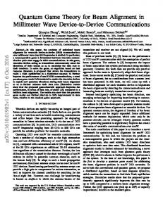
12.8% and 36.4% for the iterative algorithm with M = 4 and M = 8, respectively, compared to the bisection algorithm. Similarly, the peak throughput performance of the exhaustive algorithm is 88.3% smaller than that of the bisection algorithm.

Fig. 3: The average throughput versus sensing duration, L; γ0 = −5dB, σ = 2π, N = 50. For exhaustive search, 1 ≤ K ≤ N .

under exhaustive search is given by    N Kγ0 N −J −1 ˆ log 1 + Vˆ0 (σ, L)=E J 2 N (N − J − 1)σ ! ˆ ˆ − 1)γ0 (a) N − L N (2L < (35) log2 1 + ˆ N (N − L)σ ! ˆ ˆ 0 (b) N − ⌊L⌋ N 2⌊L⌋γ , (36) ≤ log2 1 + ˆ N (N − ⌊L⌋)σ where in (a) we used the fact that log(1 + x) is concave in x, hence its perspective function t log(1 + x/t) is concave in t > 0 [15], and Jensen’s inequality; in (b), we used the fact that ˆ ˆ t log(1+x/t) is an increasing function of t, and 2L−1 ≤ 2⌊L⌋ ˆ ˆ ˆ since L ∈ {⌊L⌋, ⌊L⌋ + 1/2}. By comparing the throughput under the bisection and exhaustive search algorithms, we obtain the following lemma. Lemma 3. The bisection algorithm strictly outperforms the exhaustive one. ˆ may not be an integer, we compare the Proof. Since L performance of exhaustive search with that of the bisection ˆ From (31) and (36), algorithm with sensing duration L = ⌊L⌋. the performance gap between the two algorithms is given by ˆ V0∗ (σ, L) − Vˆ0 (σ, L)      N 2 L γ0 N 2Lγ0 N −L log2 1+ − log2 1+ ≥0 > N σ(N −L) σ(N −L) since 2L ≥ 2L. The lemma is thus proved.



B. Numerical Results We consider the following scenario: N = 50, γ0 = −5dB, σ = 2π. In Fig. 3, we plot the throughput achieved by bisection, iterative, and exhaustive search algorithms as a function of the sensing duration L. Note that the throughput curves exhibit a quasi concave trend. It can also be noticed that the curve corresponding to the proposed bisection algorithm achieves superior performance with respect to the exhaustive and iterative search algorithms, as proved analytically. Of particular interest is to compare the ”peak” throughput of these algorithms, obtained by optimizing over the sensing duration L. We observe a performance degradation of approximately

V. C ONCLUSION In this paper, we have studied the design of the optimal beam alignment algorithm in mm-wave downlink networks, so as to maximize the throughput. We have proved the optimality of a bisection algorithm, and showed that it outperforms other algorithms proposed in the literature, such as exhaustive search and iterative search. Moreover, we have formulated an optimization problem to find the optimal duration of the sensing phase in order to maximize the throughput, and we have shown that the iterative algorithms with division factors of 4 and 8 and the exhaustive search algorithm achieve 12.8%, 36.4% and 88.3% lower ”peak” throughput than the bisection algorithm, respectively. R EFERENCES

[1] CISCO, “Cisco visual networking index: Global mobile data traffic forecast update, 2016–2021 white paper,” http://www.cisco.com/c/en/us/solutions/collateral/service-provider/visual-networking-ind [2] T. S. Rappaport, S. Sun, R. Mayzus, H. Zhao, Y. Azar, K. Wang, G. N. Wong, J. K. Schulz, M. Samimi, and F. Gutierrez, “Millimeter Wave Mobile Communications for 5G Cellular: It Will Work!” IEEE Access, vol. 1, pp. 335–349, 2013. [3] A. Ghosh, T. A. Thomas, M. C. Cudak, R. Ratasuk, P. Moorut, F. W. Vook, T. S. Rappaport, G. R. MacCartney, S. Sun, and S. Nie, “Millimeter-Wave Enhanced Local Area Systems: A High-Data-Rate Approach for Future Wireless Networks,” IEEE Journal on Selected Areas in Communications, vol. 32, no. 6, pp. 1152–1163, June 2014. [4] N. Michelusi, M. Nokleby, U. Mitra, and R. Calderbank, “Multi-scale Spectrum Sensing in Small-Cell mm-Wave Cognitive Wireless Networks,” in IEEE International Conference on Communications (ICC), 2017, to appear. [5] T. S. Rappaport, Wireless communications: principles and practice. Prentice Hall PTR, 2002. [6] M. R. Akdeniz, Y. Liu, M. K. Samimi, S. Sun, S. Rangan, T. S. Rappaport, and E. Erkip, “Millimeter Wave Channel Modeling and Cellular Capacity Evaluation,” IEEE Journal on Selected Areas in Communications, vol. 32, no. 6, pp. 1164–1179, June 2014. [7] C. Jeong, J. Park, and H. Yu, “Random access in millimeter-wave beamforming cellular networks: issues and approaches,” IEEE Communications Magazine, vol. 53, no. 1, pp. 180–185, January 2015. [8] Y. Li, J. G. Andrews, F. Baccelli, T. D. Novlan, and J. Zhang, “On the initial access design in millimeter wave cellular networks,” in 2016 IEEE Globecom Workshops (GC Wkshps), Dec 2016, pp. 1–6. [9] V. Desai, L. Krzymien, P. Sartori, W. Xiao, A. Soong, and A. Alkhateeb, “Initial beamforming for mmWave communications,” in 48th Asilomar Conference on Signals, Systems and Computers, Nov 2014, pp. 1926– 1930. [10] A. Capone, I. Filippini, and V. Sciancalepore, “Context Information for Fast Cell Discovery in mm-wave 5G Networks,” in 21th European Wireless Conference, May 2015, pp. 1–6. [11] C. N. Barati, S. A. Hosseini, M. Mezzavilla, T. Korakis, S. S. Panwar, S. Rangan, and M. Zorzi, “Initial Access in Millimeter Wave Cellular Systems,” IEEE Transactions on Wireless Communications, vol. 15, no. 12, pp. 7926–7940, Dec 2016. [12] T. Bai and R. W. Heath, “Coverage and Rate Analysis for MillimeterWave Cellular Networks,” IEEE Transactions on Wireless Communications, vol. 14, no. 2, pp. 1100–1114, Feb 2015. [13] S. Rangan, T. S. Rappaport, and E. Erkip, “Millimeter-wave cellular wireless networks: Potentials and challenges,” Proceedings of the IEEE, vol. 102, no. 3, pp. 366–385, March 2014. [14] D. P. Bertsekas, Dynamic programming and optimal control. Athena Scientific, 2005. [15] S. P. Boyd and L. Vandenberghe, Convex optimization. Cambridge Univ. Pr., 2011.