are simulated using a 1D model for the laser-matter interaction, describing ... nonequilibrium heating and vaporization of the target material, and also using a 1D multi- .... the numerical threshold is 1.7J/cm2 (113.3MW/cm2) and the experimental ...... 2.15.10−0.502. 0.12 + 7.1−5(T − Tm). Specific Heat Cp( cal. K.g. ) Solid c-.
Modeling and Numerical simulation of laser matter interaction and ablation with a 193 nanometer laser for nanosecond pulse J. D. Parisse, M. Sentis and D.E. Zeitoun Aix Marseille Universit´e, IUSTI/UMR CNRS 6595 Technopˆole de Chˆateau Gombert, 5 rue Enrico Fermi, 13013 Marseille, France and LP3 Laboratory Lasers, Plasmas and Photonic Processes UMR 6182 CNRS - Mediterranean University (Dated: November 20, 2009)
Abstract The aim of this work was to develop a new plasma creation model to complete our previous expansion model. In the past to determine the initial conditions for the expansion code we used using the FILM code. But this code is not really adapted for the fluence range we work with. Therefore we have decided to develop our own modeling and numerical code treating the plasma creation. This paper describes a new set of numerical models for the laser-matter interaction between a 193nm laser and a silicon target. A new model for the laser evaporated-matter interaction has been developed. All the models take into account the electronic non-equilibrium as well as the ionization processes and the laser beam absorption. All our calculations have been validated and compared to numerical results and even to previous plasma creation models. We have an overall good agreement with the experimental results. The comparison with experimental data has shown that we have a very efficient model for power density over 170 M W/cm2 . This is a very good improvement in comparison with the older model (as FILM for example) which is efficient over 1 GW/cm2 . PACS numbers: 47.11.+j, 47.20.Ma, 47.32.Cc, 47.40.Nm
1
I.
INTRODUCTION
Pulsed laser deposition (PLD) has become a flexible and effective method to deposit a wide variety of thin films extending from High-Tc superconductor to dielectric materials. Among the numerous parameters which affect the quality of the films, the plasma characteristics (velocity, temperature, pressure, density and composition) are very important. In spite of the considerable successes that have been achieved in making thin films by using laser ablation, the ablation process (especially the plasma creation) and the laser-induced plume dynamics expansion into an ambient gas are not fully understood. Compared to the expansion into vacuum, the interaction of the plume with an ambient gas is a far more complicated gas dynamics process which involves the deceleration, attenuation, thermalization and recombination of the ablated species, and formation of shock waves. PLD phenomena generally produced by a short laser pulse duration (ranging from femtoseconds to nanoseconds) and a relatively low laser fluence (≤ 1GW/cm2 ) can be described by four successive stages : (i) evaporation of the target material, (ii) interaction of the evaporated cloud with laser beam resulting in the cloud heating and perhaps plasma formation (figure 1), (iii) plasma plume expansion into vacuum or background gas environment (figure 2), and finally (iv) deposition of the ablated material on a substrate. PLD is not our group’s sole interest. For example another application could be surfaces cleaning, especially in order to treat surfaces contaminated by nuclear radiations. This will be a major issue when nuclear plants, will have to dismounted dismounted. PLD and laser cleaning could seem very different but in the end it is exactly the same process but with only different goals. The difference is that in laser cleaning you want to remove a film from a surface and then, in nuclear contaminated cases, collected the waste. We are associated to ONECTRA (an ONET’s branch) for these applications. This paper will deal with the first three stages of the whole process. However it is focused on the laser-matter interaction and plasma creation stages. This choice has been made because the results given by the code the FILM [1] and [2] for the fluence we work with were not in good agreement with the experimental data. The first two processes are simulated using a 1D model for the laser-matter interaction, describing the electronic nonequilibrium heating and vaporization of the target material, and also using a 1D multispecies Euler equations for the plasma creation stage including nonequilibrium for ionization processes and laser absorption (Inverse Bremstrahlung absorption and photoionization) by
2
the cloud. The third process is described by a 3D axisymmetric nonequilibrium ionized multi-species Navier Stokes equations (ref : 3). In our modeling the background gas is He or Ar, the ablated matter is silicon and the laser used is an UV excimer (ArF 193 nm, 6.4eV) one. The numerical results will be discussed and compared to the experimental ones. Throughout the paper the cgs unit system is used. The universal constants used in this paper can be found in Table I.
II.
LASER-MATTER INTERACTION
The first step of the plasma creation is the laser-matter interaction (cf figure 1), During this step the laser heats the silicon target, then it melts it and eventually evaporates it.
A.
Equations
This part of the model, which is 1D, gives the rate of evaporated matter that appears in the ambient gas. The model, which takes into account the electronic nonequilibrium effect during the silicon target heating, was developed by Van Driel [3] and is updated in this paper using Anisimovs assumption [4] for the liquid phase. In this model there are three equations : one for the free carriers density, another one for the free carriers energy and the classical heat transfer equation for the lattice temperature evolution. The equations are written as follows : for the solid Phase : ∂(Da ∂N ) ∂N ∂x = + SN ∂t ∂x α0 I(x, t) SN = + δN − γA N 3 hνlaser
(1) (2)
∂(Te Da ∂N ) ∂Ee ∂x = 3k + Se ∂t ∂x Se = θα0 I(x, t) + (γA N 3 − δN )Eg − 3kN ∂(λ ∂T ) ∂H ∂x = + Sq ∂t ∂x Te − T Sq = +3kN τe 3
(3) Te − T τe
(4) (5) (6)
where N is the free carriers (electrons and holes) density, Da is the ambipolar diffusion coefficient, α0 is the inverse absorption length also called absorption coefficient, δ the ionization impact coefficient and γA the Auger recombination coefficient, νlaser is the laser frequency, θ =
hνlaser −Eg Eg
is the effective energy gained by the free carriers during the intrinsic ab-
sorption. Eg is the silicon electronic gap. Ee is the electronic energy and Te the electronic temperature. H is the lattice enthalpy (we have chosen to work with the enthalpy in order to ease the phase change calculation) τe is the energy relaxation time between the free carriers and the lattice in the solid case and is equal to 10−13 s [3]. for the liquid Phase : ) ∂(Da ∂N ∂N ∂x = + SN ∂t ∂x α0 I(x, t) SN = hνlaser ) ∂Ee 3 ∂(Te Da ∂N ∂x = k + Se ∂t 2 ∂x 3 Te − T Se = α0 I(x, t) − kN 2 τe ∂(λ ∂T ) ∂H ∂x = + Sq ∂t ∂x Te − T 3 Sq = + kN 2 τe
(7) (8) (9) (10) (11) (12)
in its liquid form the silicon behaves like a metal so contrary to the solid phase N is only the excited electrons density, that is also why the 3kN has become 23 kN , τe is the energy relaxation time between the excited electrons and the lattice in the liquid case and is equal to 10−14 s [4]. All the silicon properties are sum up in Tables II-V, these data come from Unamuno & Fogarassy [5] and Van Driel [3]. In both cases I(x,t) is the laser intensity transmited at the x depth at the t time, the evolution I(x,t) is given by the Beer-Lambert law [3] : I(x, t) = (1 − R).I0 (t).e−α0 .x
(13)
where R is the reflectivity of the irradiated surface and I0 (t) is the incident laser intensity, in our case we have modeled the spatial evolution of the laser intensity by using a Gaussian function. It is not exactly right for an excimer pulse but, as it will be shown later, it describes correctly the laser pulse correctly. 4
B.
Boundary and initial conditions
The domain used for the calculations is big or deep enough to suppose that the end of the domain is not affected by the laser pulse, so the boundary conditions at the deep end of the domain are the initial conditions [3] : N (xend ) = N0 = N (t = 0s) = 10−12 cm−3
(14)
T (xend ) = T0 = T (t = 0s) = 300K
(15)
Te (xend ) = Te0 = Te (t = 0s) = 300K
(16)
For the surface which receives the laser flux the boundary condition used is a zero flux one for the three equations in solid or liquid phase, because there are no particle or energy fluxes until the boiling begins. ∂N )x=0 = 0 ∂x ∂T ( )x=0 = 0 ∂x ∂Te ( )x=0 = 0 ∂x (
(17) (18) (19)
When the boiling begins there is a flux of particles due to the evaporation of the Silicon target and there also are energy fluxes associated to the particles fluxes. In order to determine the boiling temperature Tm the classical Clausius-Clapeyron law is used. These fluxes will be used in the plasma creation model (paragraph III) as boundary and initial conditions.
C.
Numerical method
The equations are solved by using an explicit center finite difference scheme : second order accuracy in space and first order in time. The size of the uniform mesh and the space step are determined taking into account two characteristic lengths : for the overall size of the mesh the thermal penetration depth must be taken into account : Xth = (4.χ.t)0.5 . The Xth represents the distance which has been thermally affected by the laser irradiation, so it is useful to determine the size of the mesh. The second length that must be considered is the laser penetration depth : X0 =
1 . α0
This distance is used to determine the the space
step ∆X, in the calculation it has always been verified that the mesh was long enough to be consistent with the ”end” boundary condition. At this end the total length of the mesh is 5
2.10−4 cm and the space step ∆X = 10−7 cm. So we have a uniform mesh composed of 2000 cells. In order to preserve the stability and consistency of the numerical scheme, the time step used for the calculation ∆t is equal to 10−14 s.
D.
Results
Before going on with the laser-evaporated matter interaction and therefore the plasma creation, we have validated our model and numerical code LASERMAT. To do so several simulations have been performed and especially melting and boiling threshold calculation, the comparisons with experimental data have been made [6]. In these two cases the laser pulse was Gaussian, as it is always the case for our model, with a width at half-height of 15ns and a pulse duration of 30ns. First of all we have to precise how the numerical threshold was obtained. Melting threshold measurements carried out by Patronne [6] state that the threshold was reached when 10nm of the target have been melted.
Figure 3 shows the surface temperature and the melted
depth evolution versus time for a 400 mJ.cm−2 (26.6 MW.cm−2 ). The constant temperature zone of the melting process is observed. The the melting depth increases to 10nm, so the threshold is reached. The numerical melting threshold is 400 mJ.cm−2 (26.6 MW.cm−2 ) that is to say exactly the same value as the measured one. Before telling more about Figure 4, let’s define what the state variable is : state = 0 for the solid phase, state = 1 for the liquid phase and state = 2 for the gaseous phase. If 0 ≤ state ≤ 1 the melting (or the solidification) is going on, so the silicon is a biphasic mix of liquid and solid. If 1 ≤ state ≤ 2 the boiling (or the condensation) is going on, so the silicon is a biphasic mix of liquid and gas. The boiling threshold is defined as the apparition of the molecule of gas so it occurs when state becomes greater than 1. From figure 4 it can be seen that the numerical boiling threshold in the first case, background gas pressure equal to 400mTorr, is 750 mJ/cm2 (50MW/cm2) which is quite close to the experimental one of 700 mJ/cm2 (46.6MW/cm2) [6]. The second one, background gas pressure 1 atm, is also in good agreement with the experimental data : the numerical threshold is 1.7J/cm2 (113.3MW/cm2) and the experimental one is 1.6J/cm2 (106.6MW/cm2) [6]. As the laser-matter interaction model has been validated we were enabled to go to the next stage of our laser ablation model. The LASERMAT code is coupled to a fluid code describing the laser-evaporated matter interaction in order to create 6
the CREAPLUME code describing the laser matter interaction and the plasma creation as a whole.
III.
LASER-EVAPORATED MATTER INTERACTION
If the laser fluence is high enough we can observe a plasma creation due to the interaction between the ablated matter and the laser pulse. The plasma is considered as a five species mixture which contains : Si, Si+ (8.1eV), Si* (excited state of Si, 5eV), Ar or He and e− (electrons). The excited state choice (5eV) is the same as Liu made [7], so the Si would be ionized if it absorbed two photon (6.4 eV each). The first four species are called heavy particles. The ions number is supposed to be equal to the electrons one, so the electrons density can be easily calculated. The initial density of the excited state of Si is calculated with Boltzmann equation.
A.
Governing Equations
The plasma evolution is governed by 1D multi-species Euler equation with energy and mass source terms [8]. • the continuity equation : ∂ρi ∂ρi u + = ωi (20) ∂t ∂x where ρi is the density of the species i (i = 1 : Si ; 2 : Si+ , 3 : Si*, 4 : Ar or He , 5 : e− ), ωi is the i species mass source term and u is the velocity in the space direction x. • the momentum equation : ∂ρu ∂(ρuu + P δij ) + =0 ∂t ∂x
(21)
where P is the pressure of the gas mixture, ρ is the total density of the gas mixture and δij the Kronecker’s symbol • the heavy particles energy equation: ∂E ∂ (uE + uP ) + = ωE ∂t ∂x
(22)
where E is the heavy particles total energy and ωE the heavy particles energy source term. 7
• the electronic energy equation: ∂u ∂Ee ∂ (uEe ) + = ωEe − Pe ∂t ∂x ∂x
(23)
where Pe is the electronic pressure, Ee is the electronic energy and ωEe electronic energy source term. This system closure is ensured by the equation of perfect gases : P =ρ
R T M
(24)
where M is the molar mass and R is the constant of perfect gases. The species molar mass Mi and formation enthalpy h0i can be found in Table VI.
B.
Mass source terms
The kinetic model is derived from Rosen0 s one [9]. The source terms, appearing in equation (20) are calculated using Zeldovitch0 s approach [10] . All the following processes are taken into account : • Excitation by electronic impact : Si + e− + 5 eV ↔ Si∗ +e− During this process there is an energy exchange between the electrons and the heavy particles, in the forward case electrons give energy to heavy particles and it is the reverse in the backward case. The electronic impact excitation forward kinetic constant is : � � � � 5eV ρ1 ρ5 .N 2 5eV −12 0.5 Kf −e = 6.10 .Te 2+ exp − kTe M1 M5 kTe
(25)
where Te is the electronic temperature, k the Boltzmann’s constant, N the Avogadro’s number. The electronic impact excitation backward kinetic constant is : � � 5eV ρ3 ρ5 .N 2 −11 0.5 Ke−f = 1.8.10 .Te 2+ kTe M3 M5
(26)
• Ionisation of the excited state by electronic impact : Si∗ + e− + 3.1 eV ↔ Si+ +e− +e− As in the previous process there is an energy exchange between the electrons and the 8
heavy particles, but there also is an electrons and ions creation in the forward case and a disappearance in the backward case. The forward kinetic constant of this process is : � �2 � � IH ρ3 ρ5 .N 2 3.1eV −10 0.5 exp − Ke−i = 2.210 .Te 3.1eV M3 M5 kTe
(27)
where IH is the hydrogen ionization potential which is equal to 13.6eV. The backward kinetic constant of this process is : � �2 � �3 IH ρ3 N −25 −1 Ki−e = 10 .Te 3.1eV M5
(28)
• Photoionization of the excited state : Si∗ + hν → Si+ +e− In this case the laser gives energy to the heavy particles to create the electrons and ion. The ionization rate due to this process is : �0.5 � �3 � � � 3.1eV ρ3 N IH −18 I(x, t) Kph = 7.910 . 3.1eV hν M5
(29)
I(x,t) is the laser intensity at the x position and t time, the transmission and absorption of the laser by the ablated matter cloud will be described later. The mass source terms are written as follows : ω1 = Ke−f − Kf −e ω2 =
M2 ω M5 5
ω3 = −Ke−f + Kf −e − Kph − Ke−i + Ki−e ω4 = 0. ω3 = Kph + Ke−i − Ki−e The relation between ω2 and ω5 is due to the quasi-neutrality hypothesis.
C.
Energy source terms
Now that all the processes are described and their associated source terms detailed we can determine the energy source term associated for each process.
9
Excitation by electronic impact [9] and [10]
Eimp = (Ke−f − Kf −e ) e∗
(30)
e∗ is the excitation potential : 5 eV
Photoionization of the excited state [9] and [10]
� M3 N + e is the ionization potential of the excited state : 3.1 eV Eph = Kph I(x, t) hν − e+
(31)
Ionisation of the excited state by electronic impact [9] and [10]
erec
� �3 � � 2 M5 M3 M5 rec + Eioni = Ki−e e − Ki−e e (32) 3 N N2 is the energy gained by the electrons during the three body recombination. Its value is
given by Zeldovitch [10] and Bulgakov, Bulgakova [11] :
e
rec
−4
= 4.3.10
e
+
= 3.1.10−4 e+
with estar = 12 kTe
� �
ρ5 N M5
� 13
ρ5 N M5
� 16
1
if kTe ≤ erec ≤ estar
Te2 1
if erec ≥ estar
Te12
= e+
if erec ≥ e+
= kTe
if erec ≤ kTe
�
2e+ kTe
� 31
.
Energy exchange between the electrons and the heavy-particles [10]
This term modelled the energy exchange between electrons and heavy-particles due to elastic collision. Eech
3 = 2
�
ρ5 N M5 10
� k
Te − T τ
(33)
τ=
7.103 .Te1.5 � � 5 N lnΛ ρM 5
(34)
3.(kTe )1.5 Λ= �0.5 � 5 N 2.(4π)0.5 e3 ρM 5
(35)
τ is the electronic relaxation time. Λ is the plasma parameter which represents the number of electrons in the Debye sphere.
Inverse Bremstralhung absorption
The laser intensity transmission through the ablated cloud also follows the Beer-Lambert law [12] : I(x, t) = I0 (t).e−α.x
(36)
Io is the incident laser intensity and α the Inverse Bremstralhung absorption coefficient, which takes into account the electron-neutral and electron-ion absorptions. The electronion coefficient is the dominant one when the plasma is created but the electron-neutral absorption coefficient must be taken into account in order to describe correctly the plasma breakdown. The energy absorbed by gas cell during this process is [12] : EIB = α.Iabs
(37)
Iabs is the absorbed intensity by the cell gas : Iabs = I(x, t) − I(x + ∆x, t). As it has already been said the Inverse Bremstralhung absorption coefficient has two parts, the electronneutral one and the electron-ion one : α = αe−n + αe−i
(38)
One of the biggest problem with the Inverse Bremstralhung absorption coefficients is the wide discrepancy between the formulations found in the literature. In order to find the good ones simulations have been carried out and compared to the experimental data.
Rosen et al [9] :
−35
α = 1.37.10
λ3 √ kTe
�
ρ5 N M5
��
11
ρ5 N ρ1 N 1 + M5 M1 200
�
(cm−1 )
(39)
λ is the laser wavelength in µm.
Gremi [13] :
� �2 λ3 ρ5 N (cm−1 ) αe−i = 6.1.10 √ kTe M5 � �� �� �0.5 � � ρ5 N ρ1 N e+ 2e+ −28 2 Si Si αe−n = 7.2.10 λ hν + 1+ (cm−1 ) M5 M1 3 3hν is the ionization potential of the silicon from its fundamental level 8.1 eV. −29
e+ Si
(40) (41)
Zel’ dovitch [10] :
For this set of coefficient the αe−i from GREMI (40) is conserved but the αe−n is derived from αe−i using Zel’dovitch0 s approach [10]. � �� �� � �� 3 ρ5 N ρ1 N π 2.IH −29 λ √ (cm−1 ) αe−n = 6.1.10 √ M1 Te M5 15 3 hν + Te
(42)
In this formula the electronic temperature Te, the hydrogen potential IH and the photon energy hν are expressed in eV. In order to take into account that at high temperature a particle can emit a photon, the absorption coefficient has to be multiplied by a correction factor introduced by Rosen et al. [14] : �
� hν CES = 1 − exp − (43) kTe Taking into account the spontaneous emission coefficient CES , the laser absorbed intensity becomes : Iabs = Iabs CES
(44)
The energy sources terms are written as follows : ωE = Eech ωEe = EIB − Eech + Eioni + Eph + Eimp
D.
Numerical method
To be consistent with the expansion code [1] the LCPFCT algorithm [15] has been chosen. This choice is also due to the versatility of this numerical scheme, and its efficiency to 12
solve such problems [16] and [17] . This algorithm has been used to solve the conservation equations. This algorithm is a predictor corrector numerical scheme accurate at the 4th order in space and 2nd order in time. Once again a uniform mesh is used with a space step ∆x = 10−4 cm, in order to be consistent with the LASERMAT code the time step ∆t remains equal to 10−14 s. The length of the calculation domain is 5.10−2 cm.
E.
Boundary conditions
When there is no gas emission from the target, because of the laser irradiation, the classical wall boundary condition is used at the target / background gas interface and no reflexion (or zero gradient) one at the end of the calculation domain. In the case of evaporation from the target surface the condition at the target / background gas interface must be changed. In this case there is a gas glow emerging from the surface. To treat this problem a total balance (mass, momentum and energy) is done on the first gas cell. To determine the Si∗ density a Boltzmann distribution is assumed : � � g∗ 5eV ρ3 = 0 .exp − ρ1 g kTe
(45)
g ∗ = 6 and g 0 = 15 are respectively the statistical weight of the excited and fundamental states. As for the electrons it is assumed that the electronic temperature is equal to the temperature of the excited electrons in the liquid just before the evaporation. For the electrons number the same assumption is used, so the electrons number in the gas is the same as in the liquid during the evaporation. In some special cases the thermoemission was also modeled. The thermoemission flux is given by [10] and [18] : � � Φ 2 Jth = 120.Tes exp − (A/cm2 ) kTe s
(46)
where Φ is the work function of the material, 4.6eV for the silicon, and Tes the electronic temperature at the surface of the target. The associated Moment and Energy fluxes are also taken into account in the global balance.
13
F.
Results
To validate this model, a comparison with experimental data has been carried out. figure 5 shows the evolution of the ablated depth versus the energy density of the laser pulse. Experimental data are from Sanchez et al. [19]. The experimental conditions are : background gas He (1atm), the laser pulse is Gaussian with half height width of 23ns. In figure 5 one can see that the Rosen’s coefficients are not relevant in our case, the differences between the calculations and the experiments range between a factor 2 and a factor 4. For the Gremi’s ones the agreement is excellent for the lowest fluence (2.7 J/cm2 or (117.4 MW/cm2 ) but for the others the errors is about 60%. The last set of coefficients (Zeldo’vitch) does not describe properly the interaction for the lowest fluence but after that the agreement is excellent (4% and 15%). So the coefficients that will be used for all the others calculations are the Zeldo’vitch’s ones. These results are very similar to Liu’s one [20] who compare measurements and simulations for a 248nm excimer laser (pulse width 25ns). In both cases the ablated depth is overestimated by the simulations. This low fluence behavior is also observed at higher wavelength : 308nm in experimental data from Cultrera [21]. Some investigation about the lowest fluence was carried out to explain the differences between measurements and simulations. In order to improve the description of the laser matter interaction we have taken into account the thermoemission (46). From Figure 6 we can se that the laser absorption by the plasma cloud is bigger with the thermoemission, which is logical as the electrons density increases in the cloud. But this increase is quite small and eventually the calculated ablated depth is still 50nm, that is to say twice bigger than the measured one. So the thermoemission is not important enough for this case and the photoemission process must be taken into account to properly describe the interaction at low fluence properly. We want to say that to take into account the photo-emitted particles, a totally new model of plasma creation must developed : with de stochastic and statistical approach for the electron (Particle In Cell for example), a continue fluid description for the heavy particles and the coupling between them. To go on with the comparison with experimental data, we have made plasma creation threshold calculations. Clarke [22] says that plasma appears when the gas near the surface of the target temperature increases much more quickly than the target surface temperature. We have made calculations for background gas pressure of 10 Pa and a Gaussian laser the width
14
which is 8ns at half height. Results exhibited on figure 7 show us that for a laser fluence of 1. J/cm2 (125MW/cm2 ) the two temperatures have the same evolution. But for the laser fluence of 1.8 J/cm2 (225MW/cm2 ) the gas temperature increases drastically. So we have found a numerical threshold of plasma creation of 1.8 J/cm2 (225MW/cm2 ) which is in very good agreement with Clarkes result of 1.88 J/cm2 (25MW/cm2 ). We have now validated, at least for a fluence range, our whole plasma creation model. Thus we are now going to examine the characteristics of the plasma at the end of the laser pulse. For this study we will use the 4. J/cm2 (173.9MW/cm2 ) Sanchez et al.[19] conditions. In figure 8 we can see that, at the end of the laser pulse, the ions fraction is around 15%. Another interesting point to note is the very low value of the Si∗ density, which shows that this species is only an intermediate state in ionization scheme used for this calculation. In Figure 9, which shows us the distribution velocity versus the distance from the target at the end of the laser pulse, we can observe the acceleration of the ablated particles. After this almost linear velocity increasing phase there is a decreasing phase which shows us the background gas expansion and acceleration behind the shock wave. Figure 10 shows the temperature and electronic temperature distributions versus the distance from the target at several moments during the laser pulse. We can see that at the beginning of the laser pulse the electronic non equilibrium increases and after a while, when the density increases, the non equilibrium decreases until the end of the laser pulse. The decrease is due to the increase of mass density and so to the increase of the elastic collisions between the electrons and the heavy particles. We can now simulate the first three parts of PLD process by using the new plasma creation model and numerical code for the first two parts and using our previous expansion code [1] for the third part.
IV.
PLASMA EXPANSION
The plasma expansion begins at the end of the laser pulse. In order to describe this expansion 3D axisymetric multi-species Navier-Stokes equations are used [8], the LASERMAT numerical code provides the initial conditions for the expansion code. The gas mixture is composed of Si, Si+ , Ar or He, and e− . In this case the quasi-neutrality approximation is also made. In order to model the self electric field generated by the plasma an ambipolar 15
diffusion assumption [1] and [8] is made. To solve these equations the LCPFCT [15] algorithm is used for the convective terms and the diffusive ones are discretized by a second order finite different scheme [23] and [24]. We have made a whole simulation on the ablation process in order to obtain numerical times of flight with our complete model. Then we have compared it with the numerical results obtained by using the code FILM [2] to initiate the expansion code and the experimental data [1] and [25]. Figure 11 shows a very good agreement between the experimental time of flight of neutral atoms (Si) and the numerical ones, in the following conditions : background gas Ar at the pressure of 400 mTorr, the laser pulse is gaussian with half height width of 15ns and an energy density of 2.25 J/cm2 (150MW/cm2 ) . It can also be seen that the initial conditions given by the code FILM are not able to give good agreement with the measurements. Figure 12 also demonstrates that the agreement between the calculated times of flight and the measured ones is very good for the 5 J/cm2 (333MW/cm2 ) case.
V.
CONCLUSIONS AND PERSPECTIVES
An efficient and reliable model and numerical code simulating laser-matter interaction between a 193nm laser beam and a silicon target has been developed and validate. It takes into account the electronic non-equilibrium in the solid phase and also in the liquid one. This code has been completed with a plasma creation module which has also been validated. It takes into account the electronic non-equilibrium and also the laser beam absorption by the ablated cloud. As we had already developed an expansion code [1], we can now simulate the first three stages of laser ablation. In all the three stages the electronic non equilibrium is taken into account. The comparison with experimental data has shown that we have a very efficient model for power density over 150 MW/cm2 . This is a very good improvement in comparison with the older model (as FILM for example) which was efficient over 1 GW/cm2 . This study has shown that if we want to work with lower fluences we will have to develop a totally new model to describe photo-emitted particles.
16
VI.
ACKNOWLEDGEMENT
We would like to thanks the ONET and especially the ONECTRA branch for the support they have provided us with for for this work, we also would like to thank the Conseil R´egional Provence Alpes Cˆotes d’Azur for their financial support.
[1] H. C. Le, D. E. Zeitoun, J. D. Parisse, M. Sentis, and W. Marine : Modeling of gas dynamics for a laser-generated plasma: Propagation into low-pressure gases, Physical Review E, 62, pp 4152-4161 2000. [2] J. Virmont Mod´elisation de linteraction laser matie flux mod´er´e. Structure dun code lagrangien monodimensionnel, Laboratoire LULLI Ecole Polytechnique, Mars 1987. [3] H. Van Driel Kinetics of high density plasmas generated in Si by 1.06 and 0.53 micrometer picosecond laser pulses, Physical review B, 35, 8166 1986. [4] S.I. Anisismov and B. Rethfeld On the theory of ultrashort laser pulse interaction with a metal SPIE Vol. 3093 192-203. [5] S.Unamuno and E. Fogarassy A thermal description of the melting of c- and a- Silicon under pulsed excimer laser App. Surf. Science 36, 1, 1989. [6] L. Patrone Nano-agr´egats de silicium et de germanium pr´epar´es par ablation laser : ´elaboration et propri´et´es ´electroniques Phd thesis Universit´e Aix-Marseille II 2000. [7] C.L Liu, J.N. Leboeuf, R.F. Wood, D.B. Geohegan, J.M. Donato, K.R. Cheen and A.A Puretzky Vapor Breakdown during ablation by nanosecond laser pulses, Progress in Astronautics and aeronautics : thermal design of aeroassited orbital transfer vehicles, 96 : 3-56, 1985. [8] J.H. Lee Basic governing equations for the flight regime of aeroassited orbital transfer vehicles, Materials Research Society Symposium Proceding vol.388 (133). [9] D.I. Rosen, J. Mitteldorf, G. Kothandaraman A.N. Pirri and E.R. Pugh Coupling of pulsed 0.35 micrometer laser radiation to aluminum alloys, J. Appl. Phys., 53 (4), 3190 1982. [10] Ya. B. Zeldovitch and Yu. P. Raizer Physics of Shock Waves and High Temperature Hydrodynamics Phenomena, Academic Press, New York 1966. [11] A.V. Bulgakov and N.M. Bulgakova, J. Phys. D : Appl. Phys. 28 1995. [12] R. Singh and Narayan, Phys Rev. B 41, 8843 1990.
17
[13] A.L. Thomann, C. Boulmer-Leborgne and B. Dubreuil A contribution to the understanding of the plasma ignition mechanism above a metal target under UV laser irradiation, Plasma Sources Sci. Technol. 6 298-306 1997. [14] D.I Rosen, D.E. Hastings and G.M. Weyl, J. Appl. Phys. 53, 5882 1987. [15] E.S. Oran, J.P. Boris A Flux Corrected Transport Algorithm for solving generalized continuity equations, Laboratory for Computational Physics and Fluid Dynamics, Naval Research Laboratory Report April 1993. [16] K. Amic, A. Lebhot and J.D. Parisse Laser Sustained Plasma in a Sonic Nozzle for Fast Atom beam, Journal of Thermophysics and Heat Transfer Vol.21, No 4 p763-771, October-December 2007. [17] J.D. Parisse, D. Zeitoun, W. Marine et M. Sentis Modlisation Numrique de la formation d’un plasma induit par ablation laser UV (193nm), Journal de Physique IV Vol. 87 p111-112 (2001). [18] C. Herring and M.H. Nichols, Rev. Mod.Phys. 21,185 1949. [19] F. Sanchez, J.L. Morenza, R. Aguiar, J.C ; Delgado and M. Varela Whiskerlike structure growth on silicon exposed to ArF excimer lase irradiation, App. Phys Lett. 69 (5) 29 july 1996. [20] D. Liu and D.M. Zhang Vaporization and Plasma Shileding during High Power Nanosecond Laser Ablation of Silicon and Nickel, Chin. Phys Lett. vol. 25, No 4 (2008)1368. [21] L. Cultrera, M.I. Zeifman and A. Perrone Investigation of liquid droplets, plume deflection and a columnar structure in laser ablation of silicon, Phys. Rev B vol. 73, 075304 (2006). [22] P. Clarke, PE. Dyer, PH. Key and H.V. Snelling Plasma Ignition thresholds in UV laser ablation plumes, App. Phys; A. 69 (Suppl.), S117-S120 1999. [23] J.P. Boris, F.F. Grinstein, E.S. Oran and R.L. Kolbe NRL memorandum report 6410-93-7192, Washington DC NRL 1993. [24] E.S. Oran, J.P. Boris Numerical simulation of reactive flow, New York Elsevier 1987 [25] H.C. Le Etude num´erique et exp´erimentales de lexpansion dun plasma induit par ablation laser sous atmosph`ere neutre , Phd Thesis Universit´e de Provence, Juin 1997.
18
Figures
19
FIG. 1: Schematic description of the laser matter interaction.
20
FIG. 2: Schematic description of the plasma expansion.
21
10
1900 1700
Experimental threshold : 400 mJ/cm! 8
1300
T 6
x 1100 900
400 mJ/cm! t = 15 ns
4
700 2 500 300 0,0
5,0x10⁻⁹
1,0x10⁻⁸
1,5x10⁻⁸
2,0x10⁻⁸
2,5x10⁻⁸
Times (s)
FIG. 3: Surface temperature and melted depth evolutions versus time.
22
0 3,0x10⁻⁸
Melted depth x (mm)
Surface temperature T (K)
1500
2100
2,0 1,8
1900
T 1,6
State 1,4
1500
1,2 1300 1,0
State
Surface temperature T(K)
1700
1100 0,8 900
0,6
Pb = 400 mTorr 750 mJ/cm²
700
0,4
500 300 0,0
0,2
5,0x10⁻⁹
1,0x10⁻⁸
1,5x10⁻⁸
2,0x10⁻⁸
2,5x10⁻⁸
0,0 3,0x10⁻⁸
Time (s)
3000
2,0
T
1,8
State
1,6 1,4
2000
1,2 1500
1,0 0,8
1000
0,6
Pb = 1 atm 1.7 J/cm²
500
0,4 0,2
0 0,0
5,0x10⁻⁹
1,0x10⁻⁸
1,5x10⁻⁸
Time (s)
23
2,0x10⁻⁸
2,5x10⁻⁸
0,0 3,0x10⁻⁸
State
Surface temperature T(K)
2500
FIG. 4: Surface temperature and surface state evolutions for a background gas pressure of 400 mTorr (left) and 1 atm (right) .
24
400
Ablated depth (nm)
350 300
Zel'dovitch Rosen GREMI Experiment (Sanchez)
250 200
Pb = 1 atm , t = 23 ns
150 100 50 0 2,5
3,0
3,5
4,0
4,5
5,0
Energy density (J/cm²)
FIG. 5: Ablated depth evolution versus energy density for a background gas pressure of 1atm and laser pulse width at middle height of 23ns.
25
1,2x10⁴
Temperature (K)
1,0x10⁴
8,0x10³
6,0x10³
3
4,0x10
without thermoemission with thermoemission
2,0x10³ 0,000
0,005
0,010
0,015
0,020
0,025
0,020
0,025
Distance (cm)
1,6x10⁵ 1,5x10⁵
Velocity(cm/s)
1,4x10⁵ 1,3x10⁵
without thermoemission with thermoemission
1,2x10⁵ 1,1x10⁵ 1,0x10⁵ 9,0x10⁴ 0,000
0,005
0,010
0,015
Distance (cm)
26
FIG. 6: Heavy particles Temperature and Velocity spatial distribution at the end of the laser pulse, for a background gas pressure of 1atm and a laser pulse width at middle high of 23ns for a 2.7 J/cm2 or 117.4 MW/cm2 laser fluence .
27
FIG. 7: Target surface temperature and first gaseous grid point evolution in time for two energy density (1. J/cm2 or125MW/cm2 and 1.8 J/cm2 or 225MW/cm2 ). Background gas pressure 10 Pa and laser pulse width at middle height of 8ns.
28
1,2x10⁻³
Whole density Si Si+ He
8,0x10⁻⁴
Density (g.cm
-3
)
1,0x10⁻³
6,0x10⁻⁴
4,0x10⁻⁴
2,0x10⁻⁴
0,0 0,000
0,005
0,010
0,015
0,020
0,025
0,030
Distance (cm)
3,0x10⁻⁷
Si*
Density (g.cm
-3
)
2,5x10⁻⁷
2,0x10⁻⁷
1,5x10⁻⁷
1,0x10⁻⁷
5,0x10⁻⁸
0,0 0,000
0,005
0,010
0,015
0,020
Distance (cm)
29
0,025
0,030
FIG. 8: Spatial distribution of densities at the end of the laser pulse. Background gas pressure is 1 atm and the laser pulse width at middle height is 23ns and the energy density is 4. J/cm2 (f173.9MW/cm2 ).
30
1,4x10⁸
1,2x10⁸
Pressure(bari)
1,0x10⁸
8,0x10⁷
6,0x10⁷
4,0x10⁷
2,0x10⁷ 0,000
0,005
0,010
0,015
0,020
0,025
0,030
0,020
0,025
0,030
Distance (cm)
4,0x10⁵
3,5x10⁵
Velocity (cm/s)
3,0x10⁵
2,5x10⁵
2,0x10⁵
1,5x10⁵
1,0x10⁵ 0,000
0,005
0,010
0,015
Distance (cm)
31
FIG. 9: Velocity distribution versus distance from the target Background gas pressure is 1 atm and the laser pulse width at middle height is 23ns and the energy density is 4. J/cm2 (173.9MW/cm2 ).
32
3,0x10⁴
T 17ns Te 17ns T 20ns Te 20ns T 25ns Te 25ns
2,5x10⁴
Temperature (K)
2,0x10⁴
1,5x10⁴
1,0x10⁴
5,0x10³
0,0 0,000
0,005
0,010
0,015
0,020
0,025
0,030
Distance (cm)
3,5x10⁴
T 32ns Te 32ns T 43ns Te 43ns
Temperature (K)
3,0x10⁴ 2,5x10⁴ 2,0x10⁴ 1,5x10⁴ 1,0x10⁴ 5,0x10³ 0,0 0,000
0,005
0,010
0,015
Distance (cm)
33
0,020
0,025
0,030
FIG. 10: temperature and electronic temperature spatial distribution at several times. Background gas pressure is 1atm and the laser pulse width at middle height is 23ns and the energy density is 4. J/cm2 (173.9MW/cm2 ).
34
240
Experiment FILM + Le Créaplume + Le
220 200 180
Time (ns)
160
2,5 J/cm² Pb = 400 mTorr t =15ns
140 120 100 80 60 40 1,0
1,2
1,4
1,6
1,8
2,0
Distance (mm)
FIG. 11: Time of flight at 1 and 2 mm for an energy density of 2.25 J/cm2 (150MW/cm2 ), a background gas pressure of 400mTorr and laser pulse with a width at middle height of 15ns.
35
180
Experiment Creaplume + Le
160
Time (ns)
140
120
5 J/cm² Pb = 900 mTorr t = 15ns
100
80
60 1,0
1,2
1,4
1,6
1,8
2,0
Distance (mm)
FIG. 12: Time of flight at 1 and 2 mm for an energy density of 5 J/cm2 (333.3MW/cm2 ), a background gas pressure of 900mTorr and laser pulse with a width at middle height of 15ns.
36
Tables
37
erg Universal constant of perfect gases R= 8.314.107 ( mol.K )
Elementary electric charge Avogadro’s number Celerity of light Planck’s constant Boltzmann’s constant
e =4.803 (esu) N = 6.023.1023 (mol−1 ) c = 2.998.108 ( cm s ) h = 6.625.10−27 (erg.s) k = 1.38.10−16 ( erg s ) TABLE I: Universal constants in cgs units.
38
Reflectivity R
Solid c- Liquid 0.6
0.679
Absorption coefficient Solid c- Liquid T ≤ 1000K
α(cm−1 )
1.65.106 1.67.106
T ≥ 1000K
α(cm−1 )
1.8.106 1.67.106
TABLE II: Optical properties of Silicon under a 193nm laser irradiation.
39
6
γA ( cm s )
δ(s−1 )
3.8.10−31 3.6.1010 .exp(
−1.5.Eg kTe )
2
Da( cm s )
Eg (eV ) 1
2
T 1.16 − 7.02.10−4 − 1.5.N 3 T +1108 18( 300 T )
TABLE III: Silicon0 s electronic properties (all the temperatures are in Kelvin).
40
Melting Temperature Tm (K) 1683
Melting Enthalpy Hm ( Jg ) 2728
Boiling temperature for 1atm Tb (K) Melting Enthalpy Hb ( Jg ) 2728
13700 TABLE IV: Silicon0 s thermodynamical properties.
41
g Density ρ( cm 3)
Solid
Liquid
2.32
2.52
Solid c-
Liquid
T ≤ 1200K
354.T −1.226
0.12 + 7.1−5 (T − Tm )
T ≥ 1200K
2.15.10−0.502
0.12 + 7.1−5 (T − Tm )
Solid c-
Liquid
cal Thermal conductivity λ( K.s.cm )
cal Specific Heat Cp ( K.g )
−4
0.166.e2.375.T.10
0.25
TABLE V: Silicon’s thermal properties (all temperatures are in Kelvin).
42
g Species Molar mass Mi ( mol ) Enthalpy formation h0i ( erg g )
Si
28
1.6.1011
Si∗
28
3.36.1011
Si+
28
4.45.1011
Ar
40
0.
He
4
0.
e−
5.867.10−4
0. TABLE VI: Species constants
43