RADIOENGINEERING, VOL. 15, NO. 4, DECEMBER 2006
91
Modeling and Optimizing Antennas for Rotational Spectroscopy Applications Zbyněk LUKEŠ, Jaroslav LÁČÍK, Zbyněk RAIDA Dept. of Radio Electronics, Brno University of Technology, Purkyňova 118, 612 00 Brno, Czech Republic
[email protected],
[email protected],
[email protected] Abstract. In the paper, dielectric and metallic lenses are modeled and optimized in order to enhance the gain of a horn antenna in the frequency range from 60 GHz to 100 GHz. Properties of designed lenses are compared and discussed. The structures are modeled in CST Microwave Studio and optimized by Particle Swarm Optimization (PSO) in order to get required antenna parameters.
Keywords Horn antenna, dielectric lens, metallic lens, particle swarm optimization, rotational spectroscopy.
1. Introduction Rotational spectroscopy (microwave spectroscopy) deals with the absorption and the emission of electromagnetic radiation in the microwave frequency spectrum by molecules associated with a corresponding change in the rotational quantum number of molecules. This spectroscopy is practical in the gas phase only, where the rotational motion is quantized. The block scheme of such a rotational spectroscope is depicted in Fig. 1 [1]. The synthesizer, whose frequency is lens
amplifiers
controlled by the rubidium standard, generates a microwave signal in the frequency range of gigahertz. This signal, after its amplification and multiplication (to get a desired frequency), is transmitted by the antenna and focused by the lens. A linearly polarized wave goes through the polarization filter to the sample cell, where an analyzed gas is located. After passing the sample cell, the wave is reflected back from the roof mirror, where the polarization of the wave is changed. The reflected wave is deflected by the polarization grid, and received by the other antenna. After that, the received signal is detected and processed by the computer. Thus, the rotational (absorption) spectrum of an analyzed gas is obtained. In the paper, horn antennas [2], [3] completed by different lenses (a dielectric one and a metallic one), which can be exploited in a microwave spectroscope, are presented. These structures are modeled in CST Microwave Studio [4] and optimized by the particle swarm optimization (PSO) method [5]. Section 2 presents methods used for modeling and optimizing lenses with a horn antenna. Section 3 describes properties of an original horn antenna. In sections 4 and 5, the horn antenna completed by a dielectric lens and a metallic one is modeled and optimized to get more efficient structures. The last section concludes this paper.
polarization grid
roof mirror
multipliers
sample cell antenna lens
synthesizer antenna rubidium standard
detector
bias
GPS
lock-in amplifier
computer
Fig. 1. Block diagram of a molecular spectroscope.
oscilloscope
92
Z. LUKEŠ, J. LÁČÍK, Z. RAIDA, MODELING AND OPTIMIZING ANTENNAS FOR ROTATIONAL SPECTROSCOPY ...
where Δt is the time step the bee flies by the velocity vn+1 (1 second usually).
2. Methods for Modeling and Optimizing Horn Antennas with Lenses In order to efficiently model and optimize a horn antenna and lenses, an appropriate numerical solver and optimization method should be chosen. A numerical method has to be fast and accurate in a wide range of frequencies, and an optimization method has to be efficient. Our demands can be accomplished by CST Microwave Studio and Particle Swarm Optimization (PSO).
2.1 CST Microwave Studio CST Microwave Studio is the commercial software for solving electromagnetic structures described by Maxwell’s equations in the differential form. In CST, the finite difference time domain method (FDTD) enhanced by the finite integration technique (FIT) is implemented. Finishing a solving procedure, transient data are mapped into the frequency domain by Fourier transform, and desired parameters of the analyzed structure are obtained. In order to model and optimize the described structures, the computational kernel of CST Microwave Studio is combined with an optimization code of the PSO algorithm implemented in Visual Basic Environment of CST Microwave Studio.
2.2 Particle Swarm Optimization The particle swarm optimization (PSO) method is a stochastic evolutionary computation technique based on the movement and the intelligence of swarms [5]. Speaking about the swarm of bees, its intention is to find the best flower in a given (feasible) space.
In the case the bee reaches the border of the feasible space, the velocity vector can be reflected (orientation of the velocity vector is reverted, and the bee returns to the feasible space), absorbed (magnitude of the velocity vector is set to zero, and the position of the bee does not change), or ignored (the bee stays out of the feasible space, its objective function is not evaluated, and the bee is expected to return to the feasible space within a few iteration steps). In our case, we use 10 agents and the maximum number of optimization iterations is set to 20. When optimizing antenna lenses, the minimized objective function considers two criteria – the impedance matching (the magnitude of the reflection coefficient at the antenna input s11 is minimized), and the maximum gain in the main lobe direction
F (x ) = w f F f (x ) + wg Fg (x ) .
(3)
Here, x is the state vector of variables changed during the optimization process, Ff(x) is the cost function corresponding to impedance matching, Fg(x) is the cost function corresponding to gain maximization, and wf and wg are weighting coefficients.
3. Modeling Original Horn Antenna The geometrical size of the original antenna is depicted in Fig. 2. The antenna consists of a circular waveguide of inner diameter R1 = 4.2 mm. At the left end of the waveguide, a feeding is placed. The right end of the waveguide is expanded into a conical horn of the dimensions D = 3 mm and R2 = 10.2 mm.
Each bee remembers the position of the lowest value of the objective function (so called local minim) it reached during its fly. The lowest local minim (through the whole swarm) is called the global minim. The position of the global minim and the local one are used to determine an optimal velocity vector (direction and speed of flight) of the bee to the area of best flowers [5]
v n+1 = w v n + w1 r1 (L best − x n ) + w2 r2 (G best − x n ) . (1) The velocity in the (n+1) iteration step vn+1 equals to the velocity in the previous iteration multiplied by a weighting factor w (how quickly the speed vn is forgotten), Lbest is the position of the local minim and Gbest of the global one, xn denotes the position of the bee in the n-th iteration step, w1 and w2 are again weighting factors, r1 and r2 are random numbers from 0 to 1. When a new velocity vector of a bee is known, its new position can be computed [5]
x n+1 = x n + Δt v n+1
(2)
Fig. 2. Basic geometry of the original horn antenna.
The antenna is assumed to be fabricated from a metal (the thickness of walls is 0.3 mm). The surface of metallic walls is plated by silver in order to minimize surface losses. Results of the analysis (the return loss in the frequency range from 60 to 100 GHz, the directivity patterns at the frequencies 60 GHz, 80 GHz and 100 GHz) are depicted in Figures 3 to 6. The gain in the orthogonal direction to the aperture is 12.8 dBi at the frequency 60 GHz, 12.8 dBi at the frequency 80 GHz, and 12.2 dBi at the frequency 100 GHz. Fig. 6 shows that the impedance matching of the antenna is sufficient.
RADIOENGINEERING, VOL. 15, NO. 4, DECEMBER 2006
93
s 11 [dB] -20 -30 -40
60
70
80
90
f [GHz]
Fig. 6. Return loss of the original horn antenna.
Fig. 3. Directivity pattern of the original horn antenna at the frequency 60 GHz.
During the optimization, the state variables x = [v, d, L]T can vary within the following ranges (Fig. 7): the distance between the antenna aperture and the front surface of the lens v ∈ , the thickness of the lens in the center d ∈ , and the diameter of the lens L ∈ . The relative permittivity of Teflon is εr = 2.25 and its loss factor equals to tan δ = 0.002.
Fig. 7. Horn antenna with the dielectric lens
Finishing the optimization process, the following values are obtained: v = 5.2 mm, d = 3.6 mm, and L = 12 mm. Fig. 4. Directivity pattern of the original horn antenna at the frequency 80 GHz.
The directivity patterns are shown in Figures 8 to 10. Further, the return loss of the optimized structure in the frequency range from 60 to 100 GHz is depicted in Fig. 11. The gain in the orthogonal direction to the aperture of the antenna is 17.4 dBi at the frequency 60 GHz, 19.3 dBi at the frequency 80 GHz, and 21.2 dBi at the frequency 100 GHz. The gain was increased in comparison to the horn antenna (section 3) about 4.6 dBi for the lowest frequency, about 6.5 dBi for the central frequency, and about 9 dBi for the highest frequency of the analyzed frequency range.
Fig. 5. Directivity pattern of the original horn antenna at the frequency 100 GHz.
4. Modeling Horn Antenna with Dielectric Lens In order to obtain better performance of the horn antenna, a dielectric lens made from Teflon (PTFE) is placed in front of the aperture (Fig. 7), and the whole structure is optimized.
Fig. 8. Directivity pattern of the antenna completed by the dielectric lens at the frequency 60 GHz.
94
Z. LUKEŠ, J. LÁČÍK, Z. RAIDA, MODELING AND OPTIMIZING ANTENNAS FOR ROTATIONAL SPECTROSCOPY ...
tallic lens has been designed to be used instead of the dielectric one (Fig. 12). The lens has been assumed to be fabricated from a metal, which surface has been plated by silver.
Fig. 12. Optimized horn antenna with metallic lamellas.
Fig. 9. Directivity pattern of the antenna completed by the dielectric lens at the frequency 80 GHz.
The metallic lens is optimized together with the horn antenna. During the optimization process, the state variables x = [v, a, b]T can vary within the following ranges (see Fig. 12): the distance between the horn aperture and the front end of the lens v ∈ , the diameter of the front end of the lens a ∈ , and the diameter of the back end of the lens b ∈ . The number of lamellas N = 5, and the length of the lens L = 20 mm does not change during the optimization. After finishing the optimization process, the following values have been obtained: v = 4 mm, a = 10 mm, b = 30 mm.
Fig. 10. Directivity pattern of the antenna completed by the dielectric lens at the frequency 100 GHz.
Fig. 11 shows that the impedance matching of the structure is sufficient in the analyzed range of frequencies. s 11 [dB] -30
Fig. 13. Directivity pattern of the optimized antenna with metallic lamellas at the frequency 60 GHz.
-40 -50
60
70
80
90
f [GHz]
Fig. 11. Return loss of the horn antenna completed by the dielectric lens.
The dielectric losses of Teflon at higher frequencies are the main disadvantage of using dielectric lenses. We have therefore tried to overcome this difficulty by designing a metallic lens.
5. Modeling Horn Antenna with Metallic Lamellas In order to eliminate the disadvantages of the dielectric lens at higher frequencies (losses in dielectrics), a me-
Fig. 14. Directivity pattern of the optimized antenna with metallic lamellas at the frequency 80 GHz.
RADIOENGINEERING, VOL. 15, NO. 4, DECEMBER 2006
95
In order to achieve even stronger improvement of antenna parameters, a metallic lens has been proposed to eliminate attenuations caused by losses in dielectrics. Unfortunately, results of the numerical analysis of the developed metallic lens showed that reflections from metallic parts degrade parameters of the antenna stronger than the losses in dielectric. Dimensions of the dielectric lens are smaller compared to the metallic one, the impedance matching is better in case of the dielectric lens, and also the gain improvement is weaker (except of the frequency 80 GHz). From the listed reasons, the dielectric lens has been recommended for implementation. Fig. 15. Directivity pattern of the optimized antenna with metallic lamellas at the frequency 100 GHz.
The directivity patterns of the horn antenna completed by the metallic lens are depicted in Fig. 13 to 15. The return loss of the optimized structure in the frequency range from 60 GHz to 100 GHz is depicted in Fig. 16.
Acknowledgements The research presented in the paper was financially supported in the frame of the research project no. LC06071 Centre of quasi-optical systems and terahertz spectroscopy.
s 11 [dB]
References
-20
[1] TOWNES, C., H., SCHAWLOW, A., L. Microwave spectroscopy. Dover Publications, 1975.
-25 f [GHz]
[2] BALANIS, C. A. Antenna Theory: Analysis and Design. New York: John Wiley & Sons, 1997.
Fig. 16. Return loss of the horn antenna completed by the metallic lamellas.
[3] MILLIGAN, T., A. Modern Antenna Design. New Jersey: John Wiley & Sons, 2005.
-30
60
70
80
90
The gain in the orthogonal direction to the aperture of the structure is 13.4 dBi at the frequency 60 GHz, 20 dBi at the frequency 80 GHz, and 16.9 dBi at 100 GHz. So, the gain was again increased in comparison to the horn antenna (section 3), but the increase is smaller than in the case of the horn completed by the dielectric lens. The magnitude of the return loss does not exceed the value –10 dB. Hence, the impedance matching of antenna is sufficient but worse than for the horn antenna completed by the dielectric lens (see Section 4).
6. Conclusion In the paper, the horn antenna completed by the dielectric lens and the metallic one has been presented. These structures have been modeled and optimized in order to get a more efficient radiating structure for a microwave spectroscope. In the frequency range of the analysis (60 GHz to 100 GHz), the horn antenna completed by the dielectric lens has exhibited good impedance matching (below –20 dB in most cases) and a good gain enhancement (from 17.4 dBi to 21.2 dBi).
[4] http//www.cst.com [5] ROBINSON, J., RAHAMAT-SAMII, Y. Particle swarm optimization in electromagnetics. IEEE Transactions on Antennas and Propagation, 2004, vol. 52, no. 2, p. 397–407.
About Authors... Zbyněk LUKEŠ graduated at the Faculty of Electrical Engineering and Communication (FEEC), Brno University of Technology (BUT), in 2002. In 2006, he defended his dissertation at the Dept. of Radio Electronics, FEEC BUT. Now, he is with the Centre of quasi-optical systems and terahertz spectroscopy. He is interested in the time-domain design of broadband antennas. Jaroslav LÁČÍK graduated at the Faculty of Electrical Engineering and Communication, Brno University of Technology (BUT), in 2002. Since 2003, he has been a post-graduate student at the Dept. of Radio Electronics, BUT. He is interested in modeling planar antennas in the time- and frequency domain by the method of moments. Zbyněk RAIDA – for biography, see p. 83 of this issue.