Modeling of Scientific Images Using GMM - Radioengineering

RADIOENGINEERING, VOL. 18, NO. 4, DECEMBER 2009

579

Modeling of Scientific Images Using GMM Jan ŠVIHLÍK Dept. of Computing and Control Engineering, Institute of Chemical Technology Prague, Technická 5, 16628, Prague, Czech Republic [email protected]

Keywords Gaussian mixture model, discrete wavelet transform, moment method, ML method, dark current.

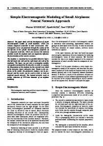
1. Introduction Various types of image models exist in the wavelet domain. A typical histogram of wavelet coefficients is shown in Fig. 1. GLM introduced [1] at the end of 80s was one of the most common used model in image denoising area. It can be expressed in the following way 

px  x  

x s

p

e Z ( s, p )

(1)

where parameter s controls the width of the PDF and parameter p controls the shape. The Z(s,p) function is given by 

Z ( s, p ) 

e





x s

p

dx 2

s 1   p  p

(2)

where Γ(x) presents the gamma function. The details about several image models in the wavelet domain can be seen in [2]. 600 500

Frequency

Abstract. This paper deals with modeling of scientific and multimedia images in the wavelet domain. Images transformed into wavelet domain have a special shape of probability density function (PDF). Thus wavelet coefficients PDFs are usually modeled using generalized Laplacian PDF model (GLM), which is characterized by two parameters. The wavelet coefficients modeling can be more efficient, while the Gaussian mixture model (GMM) is utilized. GMM model is given by addition of at least two Gaussian PDFs with different standard deviations. The equation system derived by moment method for GMM model parameters estimation will be presented. The equation system was derived for an addition of two GMM models. So it is suitable for advanced denoising systems, where an addition of two GMM random variables is considered (e.g. dark current). This paper presents a continuing of previous work [11], deals with dark current elimination (novel approach) and shows a better way of to modeling light image and dark current.

400 300 200 100 0 -200

-100

0

100

200

Magnitude of wavelet coefficients

Fig. 1. Histogram of wavelet coefficients, subband HH3, dark frame DARK_10_60_-34.fit.

Our interest lies in the area of astronomical images. The astronomical images are characterized by special image content and by a large number of bits per pixel (bpp) (commonly 14-16 bpp) in comparison with the multimedia one. These scientific data usually contain the objects (e.g. stars, nebulae, galaxies etc.), which present the subjects of interest and investigation. In the case of a night sky data acquired at low luminance, the acquiring process caused image contamination by various types of noises. This process should be modeled using Poisson noise or using addition of Poisson noise and Gaussian readout noise [3]. Furthermore, if an astronomical camera is darkened, a signal is detected at the camera output. This output signal comes from the thermally generated charge (dark current) in the crystalline lattice. Thus, considering very low temperature (approx. -100°C) of a CCD sensor the thermally generated charge becomes negligible. Hence, astronomical cameras are usually cooled to partially suppress thermal charge. A sensor cooling is often done by Peltier effect. As can be seen in Section 2, dark current can be removed by so-called dark frame. In the case of astronomical images decomposed into the wavelet domain, the wavelet coefficients occasionally do not satisfy the generalized Laplacian random variable well. This problem is caused by a sparse histogram of astronomical images in space domain. Image data with a sparse histogram cannot generate generalized Laplacian

580

J. ŠVIHLÍK, MODELING OF SCIENTIFIC IMAGES USING GMM

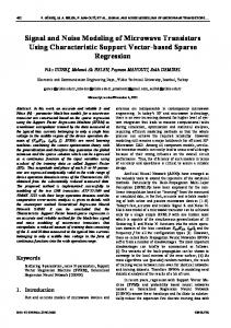
random variable correctly. A typical histogram of light astronomical image is depicted in Fig. 2. This image histogram illustrates that a dynamic range (0 – 65536) of an image is filled very sparsely. Furthermore, scientific image cannot be processed using nonlinear transfer functions to equalize histogram. Since GLM is in certain number of cases unsuitable for astronomical image modeling, we chose GMM. GMM allows to model wavelet coefficients of scientific images even in its simplest form (addition of two Gaussians).

Frequency

2

x 10

4

1.5 1 0.5

0

2000

4000

6000

8000

10000

Pixel value

Fig. 2. Histogram of 16bits light image, 2g0831a.037.fits.

2. Image Data 2.1 Scientific Image Data Scientific images with 16 bpp were chosen (fits and dat format) for the simulations. FITS (Flexible Image Transport System) is primarily designed to store scientific data sets. These scientific analyzed data has been taken during work of the international (Czech-Spanish) experiment BOOTES (Burst Observer Optical Transient Exploring System). The BOOTES [4] has been in service since 1998 as the first Spanish robotic telescope for the sky observation.

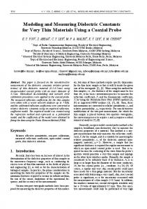
Fig. 3. Astronomical images (inverted gray scale), top: 2g980831.d00.fits dark frame, exposure time = 180 sec, CCD temperature = 4.21 °C, bottom: 1m11.01.dat light image, exposure time = 300 sec, CCD temperature = 4.21 °C.

A dark frame maps thermally generated charge [5] in the CCD sensor. It should be seen as a type of an additive noise and it should be acquired at the same conditions (exposure time, temperature) as a corresponding light image.

2.2 Multimedia Image Data The four 8 bpp testing images (non-compressed tiff format) were used in the simulations. The brada, woman, boat and cameraman image are depicted in Fig. 4.

This system is one of three similar and fully operational systems in the world. The main aim of the project is an observation of the extragalactic objects and detection of a new optical transient (OT) of gamma ray burst (GRB) sources. ASTRONOMICAL IMAGE 2dark300.000.dat 2g0831a.002.fits 2g980831.d00.fits

EXPOSURE DATE dd/mm/yyyy 19/03/1999 31/08/1998 01/09/1998

EXPOSURE TIME [sec] 1000 128 180

CCD TEMP [°C] +4.21 +4.21 +4.21

Tab. 1. Image parameters.

An example of a light image (image with objects, nebulae, stars etc.) and a dark frame (correction image) is depicted in Fig. 3. Tab. 1 contains parameters of astronomical images used in our simulations.

Fig. 4. Multimedia testing images.

RADIOENGINEERING, VOL. 18, NO. 4, DECEMBER 2009

2.3 Discrete Wavelet Transform A dyadic decomposition was used as a special form of The Discrete Wavelet Transform (DWT) in this work [1]. A Dyadic decomposition allows non redundant decomposition of a signal (in contrast to The Continuous Wavelet Transformation - CWT). An application of DWT will be denoted in accordance with Section 3.1 (i.e. DWT{.}). There is a basic structure for dyadic decomposition in Fig. 5 where Hi respectively Lo presents the impulse response of a high pass filter respectively a low pass filter, 2↓ means down sample by factor 2. If the signal is filtered using the scheme in Fig. 5 then the four subbands (matrices) are obtained, e.g. diagonal details (HH) γDp+1(d), vertical details (HL) γDp+1(v), horizontal details (LH) γDp+1(h) and signal approximation (LL) γAp+1. The matrix γA0 presents the signal which is to be decomposed.

581

In the orthogonal case, it is difficult to achieve a large number of vanishing moments and a small support size at the same time. The theoretical limit is K = 2Nv − 1 and is achieved in the Daubechies wavelets, usually denoted as dbNv. Decomposition filters [7] were estimated from the wavelet Daubechies10 and Coiflet4. The wavelet Coiflet4 gives satisfactory denoising results in the sense of MSE (Mean Square Error) [8] and the wavelet coefficients generated by wavelet Daubechies10 satisfy derived equation system well. It was found empirically.

2.4 Image Model In this paper, we consider an addition (4) of two independent random variables. Both random variables are modeled using Gaussian Mixture Model

y  x  n.

columns

Hi

rows

Hi

2

 D pd1

columns

Lo  Ap

2

2

 D pv1

2

 D ph1

columns

Hi

rows

Lo

2

columns

Lo

2

 Ap 1

(4)

Variable x presents image data and n denotes additive noise (e.g. dark current). GMM [9] is generally given by a mixture of certain number of Gaussian PDFs with variances σk and mean values μk



K



p x     k N x;  k ,  k2 .

(5)

k 1

αk are the proportions of mixture and parameter αk satisfies the constraint ΣKk=1ak=1. If k = 2, GMM is given by









p x     N x; 1 ,  12  1     N x;  2 ,  22 .

(6)

The model given by equation (6) will be utilized in this paper for image and noise modeling while μ1 and μ2 are equal to zero.

3. Model Parameters Estimation Fig. 5. Top: implementation of 2-D dyadic decomposition, bottom: magnitudes of wavelet coefficients of cameraman image, LL1 – top left, HL1 – top right, LH1 – bottom left, HH1 – bottom right.

Important tasks are which wavelets to chose and why [6]. Firstly, it is known that image denoising becomes simpler in a sparse wavelet representation (i.e. only a small number of wavelet coefficients with large magnitude). This statement [6] holds mainly for decimated wavelet transform (e.g. dyadic decomposition). Secondly, it is necessary to give attention to the image quality. Thus, the goal is to produce as many as possible wavelet coefficients that are close to zero. This depends on the vanishing moments Nv and on the support size K of the analysis wavelet. For the image quality, the regularity and symmetry of the synthesis wavelet are important.

The equation system derived by the moment method will be presented [10] and also equations derived by the maximum likelihood method [10]. Since it is problem to estimate GMM parameters of useful signal x directly from noisy observation, it is necessary to make a noise analysis. We investigated two ways how to estimate noise GMM parameters. The first method is based on statistical analysis of dark current represented by a set of dark frame images acquired at certain temperatures of the CCD sensor and the second one is based also on statistical analysis of dark frames and on Parseval’s theorem.

3.1 Moment Method The moment method, which is based on comparing of the sample moments with theoretic moments, belongs to the powerful parameters estimating methods.

582

J. ŠVIHLÍK, MODELING OF SCIENTIFIC IMAGES USING GMM

We consider additive noise in the wavelet domain Y = X + N, where X = DWT{x} and N = DWT{n}. The central theoretic moments of X is given by (7)

{ˆ12X , ˆ 22X , ˆ X } 

m4  X   3 X  14X  31   X  24X

(8)

 arg



m2  N    N  12N  1   N  22N ,

(9)

m4 N   3 N  14N  31   N  24N

(10)

where σ1N denotes the first model variance of noise and σ2N presents the second model variance. Necessary moments are derived. Now we need to find appropriate r-th theoretical moments mr(Y). If variables X and N are independent, the PDF pY of Y is given by convolution integral pY x  



 p  p x   d . X

N

(11)



Central theoretical moments of Y were derived using equation (11) m2 Y   m2  X   m2 N  ,

(12)

m4 Y   m4  X   6m2  N m2  X   m4  N  .

(13)

We derived two equations with six unknowns. Three parameters of noise GMM should be estimated using the known temperature dependency of sample moments [11]. Since we still have two equations with three unknowns, a kurtosis will be defined. Kurtosis κX is given by

X 

  2 X

The maximum likelihood estimation is given by

m2  X    X  12X  1   X  22X ,

where σ1X denotes the first model variance of useful signal and σ2X presents the second model variance. Similarly we can define central theoretic moments of noise. These moments will be practically identical with equations (7-8).

X 

3.2 Maximum Likelihood Method

4 1X

m4  X  m22  X 

(14)

3 X  14X  31   X  24X (15) 2  2 X  12X  22X 1   X   1   X   24X

where theoretical moments can be substituted by sample moments M2(X), M4(X) computed using equations (12-13). The first term after division should be equal to κX ≈ 3/αX (αX - 1 → 0). We empirically found that only this the first term after division can be used for estimation of αX. The variances σ1X and σ2X will be estimated utilizing equations (7-8)  12X 3 X  12X  6 X m2  X   (16)   X m4  X   m4  X   3m22  X   0

 22X 

m2  X    X  1X

2 1X

(17)

The parameters estimation highly depends on the estimation quality of sample moments.



max 2 2

1X

, 2 X , X

p y   N

 x  p X  x dx

k

(18)

k 

where pN denotes the noise PDF and pX presents the PDF of useful signal. The equation (18) was evaluated numerically.

4. Statistical Analysis of Dark Current 4.1 Dark Current Analysis Using Parseval’s theorem As was mentioned above we investigated two ways how to estimate noise model parameters. The first way is to make an analysis of dark frame images acquired at certain temperatures. The results of dark frame analysis can be seen in [11]. The second method based on Parseval’s theorem and also based on previous mentioned measurements on cameras is discussed in the next section. Since the stored moments dependencies are represented by a large number of values, we used the Parseval’s theorem for a problem simplification. It is generally known that a generated charge in CCD sensors depends linearly on an exposition time. The moment temperature dependency acquired at certain exposure time should be renormalized to another exposure time. Furthermore, it is possible to model temperature dependencies of second sample moment acquired at suitable exposure time and than the values of second sample moments using Parseval’s theorem in the wavelet domain evaluated. Unfortunately, the fourth sample moments have to be evaluated from measured temperature dependencies in the wavelet domain. Let be n 'i  ni  n noise with subtracted mean value and let be N 'i  DFT {n'i } noise in the wavelet domain. In accordance with Parseval’s theorem it should be written I

I

 n'   N '  2

i 1

i

i 1

2

i

(19)

where I denotes a number of matrix elements. The equation (19) caused the following moment equality I 1 I n'i 2  1  N 'i 2 .  I i 1 I i 1

(20)

If we consider iid (Independent and Identically Distributed) random variable, all wavelet subbands have the same second moment at the first decomposition level M 2 N  

I /4 1 I n'i 2  4  N 'i 2 .  I i 1 I i 1

(21)

RADIOENGINEERING, VOL. 18, NO. 4, DECEMBER 2009

583

The number of matrix elements equal to I/4 denotes that the second moment is computed in one subband only.

The results obtained by moment and maximum likelihood method applied on the GMM data contaminated by GMM will be presented. The estimated models should be compared with models estimated on data without the noise. A Jeffrey divergence was used as an evaluative criterion. The Jeffrey divergence is an empirical measure of the distributions similarity based on their relative entropy [12]. The Jeffrey divergence is given by





   pi2    pi2   ln 1 2     0 . 5 p p i i    (22)



(1)

where p denotes the model PDF and p measured data.

(2)

-2.5 -3

-150

-100

-50

0

50

100

150

x Fig. 6. Model of PDF of woman.tiff in the wavelet domain, top: subband HL3, σ1X = 124.9, σ2X = 38.3, αX = 0.20, JD = 0.0067; bottom: subband HH3, σ1X = 64.4, σ2X = 11.5, αX = 0.36, JD = 0.0102.



the PDF of

-2

-3.5

-2

Hist Model

-2.5

Log10[pX(x)]

I   pi1 JD    pi1  ln 1 2  i 1   0.5 pi  pi

Log10[pX(x)]

5. Results

Hist Model

-1.5

The proposed equation systems were tested using all testing images from Section 2.1 and 2.2. If we consider fifth decomposition level maximally (used in [11]) then we have fifteen subbands of wavelet coefficients to model (for every testing image). Hence, the next sections contain chosen results to illustrate algorithm performance.

-3 -3.5 -4 -4.5 -5 -600

-400

-200

0

200

400

600

x -2

Hist Model

5.1 Image Data (GMM) without the Noise Contamination Modeled Using Moment Method Now we consider image data without any noise contamination, because we need to know the model parameters as well as can be. In the case, the image data are without the noise, the process of model parameters estimation should be simplified using the following equality σ1X = x0.999/3, where x0.999 denotes the 99.9th percentile. The modeled PDF of wavelet subband of multimedia image can be seen in Fig. 6 and the modeled PDF of wavelet subband of scientific image can be seen in Fig. 7.

-3 -3.5 -4 -4.5 -5 -500

0

500

x Fig. 7. Model of PDF of dark frame 2dark300.000.dat in the wavelet domain, top: subband HL3, σ1X = 252.4, σ2X = 39.0, αX = 0.16, JD = 0.0042; bottom: subband HH3, σ1X = 386.1, σ2X = 54.6, αX = 0.12, JD = 0.0030.

5.2 Image Data (GMM) without the Noise Contamination Modeled Using Maximum Likelihood

Hist Model

-2

-1.5

Hist Model

-2

-2.5

Log10[pX(x)]

Log10[pX(x)]

Log10[pX(x)]

-2.5

-3 -3.5

-2.5 -3 -3.5 -4

-4 -200

-100

0

x

100

200

-200

-100

0

x

100

200

584

J. ŠVIHLÍK, MODELING OF SCIENTIFIC IMAGES USING GMM

Hist Model

Log10[pX(x)]

-1.5 -2 -2.5 -3 -3.5 -150

-100

-50

0

50

100

150

x

Fig. 8. Model of PDF of woman.tiff in the wavelet domain, top: subband HL3, σ1X = 124.9, σ2X = 24.1, αX = 0.30, JD = 0.0038; bottom: subband HH3, σ1X = 64.4, σ2X = 9.1, αX = 0.40, JD = 0.0094.

A certain image from the addition of multimedia images can be formally seen as the noise and the second one as the useful signal. The choice of so-called imagenoise is not so critical. If we chose the second image as the noisy one, the estimating process will be similar and the parameters of the useful signal will be estimated. The parameters of HH3 subband of brada.tiff are σ1N =35.6, σ2N = 4.1, αX = 0.23, JD = 0.0436 and for HL3 subband are σ1N=69.3, σ2N = 16.5, αX = 0.33, JD = 0.0786. There is the woman.tiff contaminated by brada.tiff in Fig. 10 and modeled PDF in Fig. 11.

There are the modeled PDFs of wavelet subbands of multimedia image woman.tiff in Fig. 8. Hist Model

Log10[pX(x)]

-2 -2.5 -3 -3.5

Fig. 10. Woman.tiff contaminated by Brada.tiff

-4 -4.5 -600

-400

-200

0

200

400

Hist Model

-2.5

Log10[pX(x)]

-2

-2

Log10[pX(x)]

Hist Model

600

x

-3

-2.5 -3 -3.5 -4 -200

-3.5

-100

0

100

200

x

-4 -4.5 -400

-200

0

200

400

x

Fig. 9. Model of PDF of dark frame 2dark300.000.dat in the wavelet domain, top: subband HL3, σ1X = 383.0, σ2X = 58.0, αX = 0.10, JD = 0.0026; bottom: subband HH3, σ1X = 253.3, σ2X = 43.0, αX = 0.20, JD = 0.0039.

There are the modeled PDFs of wavelet subbands of dark frame 2dark300.000.dat in Fig. 9.

5.3 Image Data (GMM) Contaminated by Noise (GMM) In the case of multimedia images, the results obtained by several methods serve mainly for algorithm optimization. The results obtained by moment method in combination with maximum likelihood method will be presented. The moment method gives an estimation of σ1X and αX and σ2X is founded using maximum likelihood. The reason of that is quite intuitive. We need to estimate three parameters, but in the case of negative numerator of (17), a standard deviation σ2X is complex.

Hist Model

-1.5

600

Log10[pX(x)]

-600

-2 -2.5 -3 -3.5 -150

-100

-50

0

50

100

150

x

Fig. 11. Model of PDF of woman.tiff estimated from addition of woman.tiff and brada.tiff in the wavelet domain, top: subband HL3, σ1X = 93.3, σ2X = 19.0, αX = 0.47, JD = 0.0027; bottom: subband HH3, σ1X = 66.3, σ2X = 11.0, αX = 0.35, JD = 0.0101.

Furthermore, another image can be added to woman.tiff and the model parameters can be estimated. Tab. 2 contains parameters of woman image estimated from addition of woman and cameraman image. There is a part of 2g0831a.002.fits image contaminated by dark frame 2g0831a.d00.fits in Fig. 12. Modeled PDF’s can be seen in Fig. 13, whereas the fit quality is satisfactory in the sense of Jeffrey divergence.

RADIOENGINEERING, VOL. 18, NO. 4, DECEMBER 2009

PARAMETERS σ1X σ2X αX JD

HL2 219 10 0.0817 0.0948

LH2 103 7 0.1495 0.0818

HH2 16 4 0.2250 0.0552

PARAMETERS σ1X σ2X αX JD

HL3 105 16 0.3879 0.0081

LH3 145 10 0.4038 0.0081

HH3 79 10 0.2363 0.0154

PARAMETERS σ1X σ2X αX JD

HL4 336 25 0.3537 0.0042

LH4 414 67 0.3494 0.0011

HH4 213 19 0.3555 0.0051

Tab. 2. Model parameters of woman.tiff estimated from addition of woman.tiff and cameraman.tiff.

585

Furthermore, another dark frame 2dark300.000.dat can be added to the light image 2g0831a.002.fits and the parameters of light image can be estimated. Parameters of chosen wavelet subbands of light image 2g0831a.002.fits estimated from the addition of 2g0831a.002.fits and 2dark300.000.dat can be seen in Tab.3. The Jeffrey divergence illustrates the quality of estimation well. PARAMETERS σ1X σ2X αX JD

HL2 1134 100 0.0130 0.0070

LH2 978 74 0.0529 0.0032

HH2 561 68 0.0338 0.0018

PARAMETERS σ1X σ2X αX JD

HL3 1094 106 0.0308 0.0021

LH3 1543 100 0.1760 0.0036

HH3 724 100 0.0482 0.0026

PARAMETERS σ1X σ2X αX JD

HL4 1224 100 0.0783 0.0030

LH4 2982 139 0.2941 0.0027

HH4 734 121 0.1300 0.0014

Tab. 3. Model parameters of light image 2g0831a.002.fits estimated from addition of 2g0831a.002.fits and 2dark300.000.dat.

6. Conclusion Fig. 12. Cut of 2g0831a.002.fits contaminated by cut of dark frame 2g0831a.d00.fits.

Hist Model

Log10[pX(x)]

-2.5 -3 -3.5 -4 -4.5 -1500 -1000 -500

0

500

This paper showed the possibilities of GMM for scientific and multimedia images modeling. Furthermore, the moment equations were derived for the case of addition of two GMM random variables. Hence, the statistical analysis of dark current was done and the algorithm for second moment evaluation based on Parseval’s theorem was proposed. The presented results have shown that our algorithms can be used for scientific and multimedia image data modeling. Proposed algorithms can be used also for dark current elimination, while the Bayesian estimators are utilized [11].

1000 1500

x

Hist Model

Log10[pX(x)]

-2.5 -3

Acknowledgements This work has been supported by the research project MSM 6046137306 of the Ministry of Education, Youth and Sports of the Czech Republic.

-3.5 -4 -4.5 -1000

-500

0

500

1000

x

Fig. 13. Model of PDF of 2g0831a.002.fits estimated from addition of 2g0831a.002.fits and 2g0831a.d00.fits in the wavelet domain, top: subband HL4, σ1X = 1085, σ2X = 142, αX = 0.12, JD = 0.0016; bottom: subband HH4, σ1X = 680, σ2X = 121, αX = 0.13, JD = 0.0012.

References [1] MALLAT, S. G. A theory for multiresolution signal decomposition: the wavelet representation. IEEE Transactions on Pattern Analysis and Machine Intelligence. July 1989, vol. 2, no. 7, p. 674 - 693.

586

[2] SRIVASTAVA, A., LEE, A. B., SIMONCELLI, E. P., ZHU, S. C. On advances in statistical modeling of natural images. Journal of Mathematical Imaging and Vision. 2003, vol. 18, p. 17 - 33. [3] STARCK, J. L., MURTAGH, F., BIJAOUI, A. Image Processing and Data Analysis: The Multiscale Approach. Cambridge University Press, 1998. ISBN 0521599148. [4] POSTIGO, A., SANGUINO, T. J., CERÓN, J. M., PÁTA, P., BERNAS, M. Recent developments in the BOOTES experiment. In AIP Conference Proceedings 662. Cambridge: Massachusetts Institute of Technology, 2003, p. 553 - 555. ISBN 0-7354-0122-5.

J. ŠVIHLÍK, MODELING OF SCIENTIFIC IMAGES USING GMM

[10] PAPOULIS, A., PILLAI, U. S. Probability, Random Variables and Stochastic Processes. McGraw-Hill, 2002. [11] ŠVIHLÍK, J., PÁTA, P. Elimination of thermally generated charge in charged coupled devices using Bayesian estimator. Radioengineering. June 2008, vol. 17, no. 2, p. 119 - 124. [12] SMITH, P., SINCLAIR, D., CIPOLLA, R., WOOD, K. Effective Corner Matching. In Proceedings of the Ninth BMVC 98. Cambridge: Massachusetts Institute of Technology, 1998.

[5] BUIL, CH., CCD Astronomy. 1st English ed. Willman-Bell, Inc, 1991. ISBN 0-943396-29-8. [6] PIZURICA, A. Image Denoising Using Wavelets and Spatial Context Modeling. PhD thesis. University Gent, 2002. [7] STRANG, G., NGUYEN, T. Wavelets and Filter Banks. 2nd ed. Wellesley-Cambridge Press, 1996. ISBN 09614088-71. [8] ADAMS, N., JIANLONG, CH., OLAFSSON, V., CHUNYU, Y. Denoising Using Wavelets. University of Michigan, 2001. [9] SAMÉ, A., OUKHELLOU, L., C ME, E., AKNIN, P. Mixturemodel-based signal denoising. Advances in Data Analysis and Classification. Springer, March 2007, vol. 1, no. 1, p. 39-51.

About Authors ... Jan ŠVIHLÍK was born in Pardubice, Czech Republic, in 1981. He received his M.Sc. from the Czech Technical University in Prague (CTU), in 2005 and Ph.D. from the CTU, in 2008. Now he is an Assistant Professor at the Institute of Chemical Technology Prague. His research interests include image processing, image denoising and statistical models of images.