Modeling and Prediction of Pedestrian Behavior based on the Sub-goal Concept Tetsushi Ikeda, Yoshihiro Chigodo, Daniel Rea, Francesco Zanlungo, Masahiro Shiomi, Takayuki Kanda Intelligent Robotics and Communication Laboratories, ATR, Kyoto, Japan E-mail:
[email protected] Abstract— This study addresses a method to predict pedestrians' long term behavior in order to enable a robot to provide them services. In order to do that we want to be able to predict their final goal and the trajectory they will follow to reach it. We attain this task borrowing from human science studies the concept of sub-goals, defined as points and landmarks of the environment towards which pedestrians walk or where they take directional choices before reaching the final destination. We retrieve the position of these sub-goals from the analysis of a large set of pedestrian trajectories in a shopping mall, and model their global behavior through transition probabilities between sub-goals. The method allows us to predict the future position of pedestrians on the basis of the observation of their trajectory up to the moment.1 Keywords-component; pedestrian models; sub-goal retrieval; behavior anticipation
I.
INTRODUCTION
A robot operating in an environment where a significant number of pedestrians is present, such as a shopping mall, needs a considerable amount of information about the current and general behavior of pedestrians in the environment. For the task of navigation, besides the obvious need to know the positions and velocities of nearby pedestrians for local planning, also the global planner can take advantage of prediction of human behavior. Knowledge of the current pedestrian density at larger distances, the average behavior of pedestrians in the environment, and even the use of a pedestrian simulator to predict the future behavior of the crowd as a whole may prevent the robot to end in highly populated areas where collision avoidance could not be performed effectively. To provide services such as guiding [1,2], surveillance, shopping assistance [3], giving information [4,5,6], assisting people who get lost, an ability to recognize behavioral patterns and predict future behavior and position is needed. In this work we tackle the problem of position prediction, which is of particular importance for a mobile robot providing services in a shopping mall. An ability of predicting the position of pedestrians beyond velocity projection will enhance the collision avoidance of the robot [7], and enable approaching humans to talk with them and providing services [8,9]. In particular, we develop an approach that gives us information useful not only for prediction but also for robot navigation, environment modeling and pedestrian simulation. To do that we use the concept of sub-goals, i.e. we assume that pedestrians have the tendency to segment the walking route to 1
This research was supported by JST, CREST.
Figure 1. Sub-goal: a point in a space pedestrians are walking towards The subgoals in the picture are retrieved with our method, see fig. 10
their final destination in a polygonal line passing through some points known as sub-goals [10,11] (Fig. 1). We assume that the position of these sub-goals is to a certain extent common to all pedestrians, i.e. that they are determined mainly by the environment. We retrieve the position of these sub-goals from the observation of a large number of trajectories, and build a probabilistic transition model between sub-goals that is used for motion prediction. The sub-goals could be used both as the nodes of the robot global path planner, and as the nodes of the planner in the pedestrian simulator, introducing a common knowledge of the environmental features based on the actual motion of pedestrians. II.
RELATED WORK
The simplest method to predict the motion of a pedestrian is to perform a velocity-based linear projection, i.e. assuming that people keep moving with a constant speed. This is known to be a reasonable approximation for short-term behavior, used for collision avoidance [12,13] and tracking algorithms [14]. The method does not need any knowledge about the environment or the previous trajectory, but it is not reliable for long term prediction ignoring environmental constraints or influence . In order to predict the future position of a walker using the information based on the previously observed behavior of a large number of pedestrians, the motion can be modeled through transitions among grids or nodes [15,16]. Recent approaches often retrieve typical transition patterns (patternbased approaches) to use also knowledge about the previous behavior of the pedestrian whose motion is being predicted [7]. The future course of a new observed trajectory is estimated with transition patterns that resemble the new trajectory [17]. Pattern-based methods use a discrete space description. Usually both for robot navigation and pedestrian simulation a continuous description in which the nodes of the global path planner are given at arbitrary distance is preferred. The usual
Figure 2. Model of a global behavior: a pedestrian follows a series of subgoals while avoiding collision with others
way to do that in robotics is to build a topological map from the geometrical features of the environment. These topological methods do not use information coming from human behavior, and though effective for navigation, they do not provide any knowledge about human behavior to the robot system [18]. Bennewitz et al. [7] use a stop point approach, i.e. retrieve the position of the nodes based on observation of human behavior, computing them as the places where people usually stop. This approach could be limited in the description of an environment in which people take decisions or just change direction without stopping. Once the graph is built with topological or humanmotion based approach, the nodes are used as the states of a hidden Markov model, and the transition probabilities are used to model and predict human behavior. In this work in order to build the nodes of the transition model we use the social science concept of “sub-goal”. The route of pedestrians can be modeled as a succession of decision points, which are influenced by the structure of the environment, as for example by the presence of landmarks and architectural features [10,11,19]. By learning from people’s trajectories, we retrieve the sub-goals from the directions pedestrians mostly head to. To reduce the effect of local dynamics, this direction to the sub-goal is computed subtracting the effect of local collision avoiding as predicted by the Social Force Model specification introduced in [20]. III.
OVERVIEW OF THE MODEL OF PEDESTRIAN BEHAVIOR
This section provides a short overview of the model of pedestrian behavior we propose (figure 2). A. Final destination (goal) We assume that pedestrians move towards a final destination, their goal. In an ideally uniform environment, without any kind of fixed or moving obstacle, neither different architectural features and the like, pedestrians would move straight to their goal. In a real environment, the goal is usually not reachable on a straight path due to the presence of fixed obstacles, and paths different from the straight one could be preferred due to easiness of walking (nature of terrain, architectural features, crowding). B. Influence of the environment (sub-goals) We assume that in a real environment pedestrians try to divide their path (global path planning) in straight segments joining their actual position with the goal [21], and we assume
Figure 3. Overview of computation in the proposed method
the nodes of these segments to be common to all pedestrians, i.e. to be determined only by the nature of the environment. Since the path to the next node is straight, these nodes are called sub-goals. These sub-goals can be determined by the presence of a visual landmark, and pedestrians may switch to their new sub-goal when it is visible to them, even before reaching the one they were walking to. C. Influence from other pedestrians (local behavior) Deviations from the straight path to next sub-goal are due to the collision avoiding (local path planning) behavior. This interaction can be expressed in a simple mathematical form applying the Social Force Model [22] (SFM), that expresses the acceleration of pedestrians as
a(t )
v p v (t )
f
j (t )
(1)
j
Here v p , stands for the preferred velocity of the pedestrian, whose magnitude is determined by the most comfortable speed for the pedestrian, and the direction by the unit vector pointing from the current position to the next sub-goal; is the time scale for the pedestrian to recover her preferred velocity, while f j is the collision avoiding behavior towards pedestrian j (the force depends on the relative positions and velocities of pedestrians). Different specifications of f have been proposed, and we adopt the specification and parameters proposed in [19], which have shown to best describe pedestrian behavior in the SFM framework. We use the SFM framework because eq (1) can be easily arranged as
v p v (t ) (a(t )
f (t )) j
(2)
j
in order to obtain v p , i.e. the direction to the next goal, from pedestrian positions, velocities and accelerations. IV.
PREDICTION ALGORITHM
A. Overview Figure 3 shows the architecture of the proposed method, which consists of an offline analysis step and an online prediction step. In the offline analysis step, from the positions and velocities of a large number of pedestrians we compute the
preferred velocities using eq. (2). Then the sub-goals in the environment are estimated by extracting points toward which many pedestrians head. In the proposed model, each pedestrian is considered to head towards one of the sub-goals and sometimes switch to a different one. So we represent each trajectory by a sequence of sub-goals, and obtain a probabilistic sub-goal transition model from observed trajectories .
a) Observed trajectories of pedestrians that go across a grid square.
In the online step, after observing the initial portion of a trajectory, we compute the preferred velocity with eq. (2). On the basis of the preferred velocity and sub-goal sequence of a pedestrian up to the moment, we estimate future positions using a probabilistic transition model. B. Estimating sub-goals After collecting a large amount of trajectories in the environment, and computing the preferred velocities, we divide the environment in a discrete grid and study the distribution of preferred directions for each grid cell. We retrieve sub-goals as points towards which a large number of directions converge, and in order to find them we define a “sub-goal” field extending the direction probabilities from each grid cell and defining the sub-goal set as the set of maxima of the sub-goal field. 1) Computing Directions of Pedestrian Motion on a Grid We discretize the environment using a square grid with linear dimension 0.5 meters which roughly corresponds to the size of a human being, and thus to the scale at which we can expect behavioral variation. For each grid the distribution of preferred directions p is obtained from velocities v p .The distribution of directions at each grid square may consist of several different components. Figures 4 (a), (b) show the observed direction distribution in a grid square. We call each component flow, and we model its angle distribution using a von Mises distribution [23],
exp( cos( )) ( | , ) 2 I 0 ( )
(3)
b) The solid line shows the histogram of directions θ, and the dashed lines show each component in the estimated von Mises mixture distribution.
c) Estimated major flow directions the grid square. The directions of the arrows correspond to the mean of the estimated von Mises distribution in b). Figure 4. Observed trajectories and the estimated flow directions in a grid square.
Figure 5. Extention of flows from grid cells. (+) represents a point where two flows cross, which is a position many people head toward and is a sub-goal candidate.
1 2 where is the mean, is the variance and I 0 ( ) is the 0 order modified Bessel function of first kind [24]. Eq. (3) gives the approximation of a Gaussian wrapped on the circle. Subsequently we estimate each component using an EM algorithm. We first discretize and smooth the direction distribution on the grid cell, and then compute the number of local maxima of this distribution. We assume that to each local maximum corresponds a flow, and fix the parameter to the position of the local maximum, and to the width of the peak around the maximum. After this initialization process, each pedestrian direction is associated to one of the von Mises mixture components according to the probability the component assigns to that direction. Then each distribution component is estimated based on the assigned pedestrian directions. This process is repeated until the estimated component has converged [25].
Figure 6. Contribution of a flow to the field
( x) .
This process defines the set of flows F { j } , i.e. the set of all the von Mises components found in the environment, each one characterized by its and values. Figure 4 (c) shows the estimated flows detected in an observed area. 2) Estimating Sub-goals from Motion Directions By extending flow directions from each grid, we can define a scalar “sub-goal” field on the environment. As shown in figure 5 in the case of two grid cells, a maximum of this field is a place in the environment towards which many people head, i.e. a sub-goal. We define the scalar field generated by the flow j in point x as
j (x) j ( | , ) ;
arg(x c)
(4)
C. Modeling Global Behavior Given a set of sub-goals, we model each pedestrian's trajectory as a sequence of movements toward one of the subgoals. So we model the long-term behavior of pedestrians by conditional probability distribution of the transition to the next sub-goal.
sub-goal sequence at each time instant (●): 1 1 1 3 2 2 2 smoothed sub-goal sequence: 1 1 1 1 2 2 2 series of sub-goals: 1 2 Figure 7. Estimating the sub-goal that a pedestrian heads towards.
where and are the parameters of the flow according to eq. (3). is the direction of the displacement vector from the grid center c, where the flow is defined, to x (Figure 6), while arg() returns the angle of the given vector. The scalar field generated by a sub-set of flows Fi F is defined as
(x; Fi )
j
( x)
(5)
j s.t. j Fi
and, following the example with two flows of figure 6, a subgoal s generated by a flow set Fi is the maximum of field (5),
s i argmax (x; Fi ) .
(6)
x
Equation (6) defines a set S {s i } of sub goals given a partition of flows {Fi } , with Fi F j and Fi F . At the same time, we define a flow partition from a sub-goal set saying that
Fi { j | s i argmax j (s k )} .
(7)
sk S
In the following we assume N sub-goals to be present in our environment, and thus the set of flows F to be divided in N subsets Fi . Our algorithm applies iteratively eqs. (6) and (7) in order to find the flow partition {Fi } and sub-goal set S that maximize
(s ; F ) i
i
(8)
si S
The algorithm is initialized searching for sub-goals on the discrete grid flows are defined on. At the beginning the flow partition consists of the whole set, F1 F , and the first subgoal s1 is the maximum on the grid of (x; F ) . The second subgoal s 2 is obtained as the point on the grid that, after obtaining the partition {F1 , F2 } from eq. (7), maximizes eq (8), i.e. (s1 ; F1 ) (s 2 ; F2 ) . The process is continued until N sub-goals and flow partitions are obtained, and at this point, using a local Monte Carlo search, eq. (6) is used to obtain the sub-goal positions in continuous space, which ends the initialization process. Subsequently, eqs. (7) and (6) are applied until convergence, i.e. the total displacement of sub-goals under application of eq. (6) is smaller than a given threshold.
1) Computing a series of past sub-goals from a fullyobserved trajectory To compute the series of sub-goals from a trajectory, first we estimate the sub-goal of the pedestrian at each instant t based on the preferred velocity. When the pedestrian is at position x with preferred velocity v p , the sub-goal with closest angle to v p that exists in a visual cone area C is selected ( y1 in Figure 7) as
s t argmin(angle( v tp , y j x t )) ,
(9)
y j in C
where angle( x , y ) is a function that returns the angle between vector x and y in [0, ] . The area of the visual cone is defined relative to x and v p and its size set to 40 degrees in angle, a value close to the typical flow spread. Then we smooth the sub-goal sequence {s t } obtained at ~ the previous step into { st } by selecting the most frequent index that appears in a fixed length time window:
~s mode(s t t / 2 ,, s t / 2 ) ,
(10)
where mode( ) is a function that returns most frequent value and is the length of the time window, set as 2000 msec, a value empirically chosen to smooth noise without losing information. Finally we compute the sub-goal series which is defined by the first sub-goal and the sub-goals that are different from the previous one (fig. 7): series of sub-goals = {~ s1} { ~st | ~st ~st 1} .
(11)
2) Transition probability To model common movements in an environment, we construct a statistical model of sub-goal transitions. We compute the following transition probabilities based on observed trajectories. p ( y 2 | y1 ) =
# of pedestirans that go toward y 1 then y 2 # of pedestirans that go toward y 1
(12)
We also compute transition model with n-1 step histories (n-gram model) p ( y N | y 1 , , y N 1 ) =
# of pedestrian s that go toward y 1 , , y N # of pedestrian s that go toward y 1 , y N 1
(13)
We computed these transitions for values of n up to 6, a compromise between computational economy and completeness of description of the environment. D. Prediction of Future Movements After observing trajectories of pedestrians up to now, our algorithm predicts future trajectory of each pedestrian.
1) Estimating the probability of the current sub-goal from a partially observed trajectory From the observed trajectories, the preferred velocity vector v p and sub-goal sequence until now {q k } are computed for each pedestrian. Suppose v p | v p | is the preferred speed, and p arg( v p ) is the preferred direction. Based on Bayes' Theorem, we model the probability that the pedestrian heads toward sub-goal y given the preferred velocity and the subgoal sequence as: p (y | , {q k }) p ( | {q k }, y ) p (y | {q k }) . p
p
(14)
The first term of the right hand side of the equation is the probability of the preferred direction p given {q k }, y , which is empirically derived from a large amount of observed trajectories. In this paper, we approximate this term assuming dependence on only the last sub-goal q m , and model the term using a Gaussian distribution, whose mean and variance depend on q m , y and are determined on empirical data. The second term is from the probabilistic sub-goal transition model. Eq. (14) is computed for all sub-goals y in the visual cone. 2) Prediction of future positions The probability that the pedestrian reaches a sub-goal z in future via any other sub-goal y i is given by p (z | p ,{q k })
p ( z |
p
,{q k }, y i ) p( y i | p ,{q k }) . (15)
i
In the following we will assume that the transition probability from y i to the next sub-goal is independent from the current preferred direction, so that the first term in the summation is simplified as p ( z | p , {q k }, y i ) p ( z | {q k }, y i )
(16)
To compute this term we sum over all the possible routes from y i to z , but since our goal is to estimate the position of a pedestrian at T seconds after the last observation, we take in consideration only the routes that are compatible with the length a pedestrian can walk in time T . Explicitly we assume p (z | {q k }, y i ) =
p(z,{r } | {q }, y ) k
k
i
{rk }L
{r k }: subgoal sequence from y i to z L : set of {r k } s.t. dist ( x, y i , r1 , , rn ) v pT and dist ( x, y i , r1 , , rn , z ) v pT where dist (r1 , r2 , ) is the distance
Sum of the length of solid lines =
v pT
Figure 8. Computation of the estimated position at time T. The lines from x to z show the sequence of sub-goals with the highest probability. Note that pedestrian changes sub-goals before reaching them. We use statistics of the distance from each sub-goal to change sub-goals.
Number of pedestrians Length of observations Size of observation area
12003 7 hours 860 m 2
Figure 9. Experimental environment。Pictures of the environment are visible in figures 1, 14.
The future position of the pedestrian at time T after the observation is estimated assuming that with probability (15), (i.e. the one that sums over the whole set L in (17)) the pedestrian will be located on the line connecting the sub-goal succession {r k } that assumes maximum probability in L , and more precisely, it will be located between sub-goal rn and subgoal z at a distance v pT ( v p is the preferred speed at x ) from x on that line, see Figure 8. V.
RESULTS
This section illustrates the model obtained with our method and compares the prediction results with those of other methods. In section V-B, to evaluate the locations of nodes, we compared our method with other node generation methods by running the same prediction procedure described in VI-C and VI-D. Then in section V-C, we further compared our method and different prediction methods.
(17)
along the route (r1 , r2 , ) x : current position of the pedestrian v p : preferred velocity T : time elapsed
where the probabilities in the summation term are obtained recursively from eq. (14). Finally, the probability to reach subgoal z given the observed sub-goal sequence and present preferred velocity, eq. (15), is obtained summing over all possible sub-goals y i in the cone of vision (using eq. 14)
A. Environment and setup We collected trajectories in a large shopping mall (Fig. 9) in which several restaurants and shops are present. Since it is located between another large building and a train station, it is a transition place for many pedestrians. The size of the observation area is 860 square meters and we observed 12003 pedestrians in 7 hours, of which 85% were used for calibration and 15% for testing. To track the pedestrians we used twenty LRFs (Hokuyo Automatic UTM-30LX) and applied a tracking algorithm based on shape-matching at torso-level [26]. This area is larger than those investigated in previous literature works, and thus the prediction task is harder.
B. Description of the environment through the sub-goal positions In this section we compare the proposed method with other methods that provide a description of the environment based on a graph, as topology based [18] methods and stop point [7] methods. The comparison is performed from a qualitative point of view, comparing the description of the environment given by the position of the nodes, and from a quantitative point of view, comparing the precision in the prediction of future positions. The topology method is implemented obtaining the map of the environment from the pedestrian movement data. The environment is discretized using a grid, and the grid cells are divided between those on which pedestrian data was recorded, and those without pedestrian data. After a smoothing process, the boundaries between the two areas are used as the boundaries of the map of the environment. In order to build the map a Voronoi diagram method [27] is applied. Also to implement the stop-point method we divide the environment using a discrete grid, and after defining the number of stoppoints N, we have check the positions of the N cells where pedestrians stop more often. After obtaining the position of the nodes, in order to predict the future position of the pedestrians we use the same method we describe in section IV-C. To estimate the future position of the pedestrian after T seconds, we select the sequence of sub-goals that has the highest probability according to Eq. (18). Then as in figure 8 we compute the point on the lines that connect the maximum probability sequence of sub-goals located at distance v pT from
a) Modeled global behavior with the proposed method.
b) Initial position of sub-goals that are placed at local peaks of eq.(6). Figure 10. (a) Modeled global behavior in the shopping mall A. Filled circles represent sub-goal positions. The sum of transition probabilities between two sub-goals is represented as the color and the width of the link. Only links with transition probability > 0.1 are shown. N=25. (b) Initial positions of subgoals.
the start point. In figures 10, 11, and 12 we show the position of the nodes in, respectively, the proposed method, the topology method and the stop point method. From a qualitative analysis, we can see that the sub-goal method depicts that pedestrians mainly just pass through the environment (14-7-3-1-10-9-0-23-17-20-2) but some of them deviate from the main corridor to go to shops (8,13,18), exhibits (16, 21) or gates (4,5). The topology method extracts nodes on crossing points between corridors (18,22,24), but other qualitatively meaningful points such as gates or entries of shops are not extracted. The stop point method has the opposite characteristic: it extracts points close to gates and shops (10,20), but this method cannot extract very well points on the corridors. We also notice that the topology method seems sometimes redundant in the description of the environment, presenting often points very close between them, something that does not occur with the proposed method.
Figure 11. Graph nodes obtained with the topology method. N=33.
Figure 12. Graph nodes obtained with the stop point method. N=25. : Proposed : Stop point
Figure 13 shows an example that illustrates this difference. The area shown in the picture connects the long corridor and the hallway space, and thus is a place where people are expected to change walking direction. The yellow lines visible on the floor are studded paving blocks located on the typical walking course to help the visually impaired, and we observe that usually also healthy people walk nearby these lines. Thus, the sub-goal point 0 is exactly the point in which we expect people to change their course. When a person comes from the corridor (right side in the picture), she typically changes her walking direction around the point 0 towards the direction of sub-goal 9. Also people coming from the hallway (left side in the picture)
20 0 10 9
Figure 13. Sub-goals and qualitative points on the main corridor
directed to the corridor usually change their moving direction at the entrance of the corridor, i.e., around sub-goal 0. This illustrates that sub-goals are extracted in the areas people typically go towards, and where they change their course.
On the other hand, the topology and stop point methods could not extract such points. The former method provides the connection points of each corridor in an environment, but not those that describe minor deviations in proximity of shops and the like. Similarly, the stop point method could not extract the points that represent walking routes through the corridor, and mostly extracted only points close to the shops (10 and 20 in Fig. 13). This method provides specific points where people rest, but not points people move towards. Judging from this qualitative comparison, we think that only the proposed method could extract all the important nodes of the environment in a compact (not redundant) way. We also compare the precision in the prediction of future positions, which we believe to be a reasonable quantitative estimation of the capability of methods to describe the motion of pedestrians. For this purpose, we measure the ratio with which the correct position of the pedestrian is within 5m from the estimated position after T seconds (given the dimension of the environment, a 5 meters error is compatible with a correct prediction of the area of the environment the pedestrian is located in, 5 meters being roughly the width of the long corridor). Each test trajectory is observed for 10 seconds (up to time t 0 ), and all methods are used to predict the position at t 0 T , for different values of T (see figure 14 for a trajectory prediction using the proposed method1). Figure 15 shows the prediction ratios for all methods. The proposed method performs clearly better than the stop point method, with a difference that grows with T , and slightly better than the topology method. To compare the performance statistically, we used a Chi-square test. The comparison with the stop point method revealed significant differences (p