Abstract. The present work describes the architecture and data flow analysis of a highly parallel processor for the Level 1 Pixel. Trigger for the BTeV experiment ...
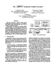
Data flow analysis of a highly parallel processor for a Level 1 Pixel Trigger G. Cancelo*, E. Gottschalk*, V. Pavlicek*, M. Wang*. J. Wu* * Fermi National Accelerator Laboratory Abstract The present work describes the architecture and data flow analysis of a highly parallel processor for the Level 1 Pixel Trigger for the BTeV experiment at Fermilab. First the Level 1 Trigger system is described. Then the major components are analyzed by resorting to mathematical modeling. Also, behavioral simulations are used to confirm the models. Results from modeling and simulations are fed back into the system in order to improve the architecture, eliminate bottlenecks, allocate sufficient buffering between processes and obtain other important design parameters. An interesting feature of the current analysis is that the models can be extended to a large class of architectures and parallel systems. I. BTeV Level 1 Trigger Fermilab’s BTeV experiment has been proposed with a Trigger System in three levels [1]. The Level 1 trigger will perform calculations using data from two detector systems: the pixel detector and the muon detector. The Level 1 must do crude data preprocessing plus Track and Vertex reconstruction while keeping the processing time as low as possible. Level 2 and 3, based on events that passed Level 1, will gather information from the already mentioned subdetectors plus other sub-detectors to perform full pattern recognition. The Level 1 Trigger process all events generated by collisions of protons and antiprotons in the Fermilab’s Tevatron. The average event interarrival time is about 132 ns at a luminosity of 2 x10 32 cm −1 s −1 . Since the Level 1 processing time will be approximately three orders of magnitude longer, the Level 1 processor will pipeline and process many events in parallel. Figure 1 shows the L1 Trigger building blocks. The Data Preprocessors have two main building blocks, the Pixel Preprocessor and the Segment Tracker. The Pixel Preprocessor formats and sorts the raw data coming from the Pixel Detector. There are two main modules in the Pixel Preprocessor, the x-y coordinate translator (XYPC) and the Time Stamp Sorter. The XYPC module formats the data; converting groups of Pixel Detector raw hits into x-y coordinate referenced data. The data generated every bunch crossing (BCO) of the accelerator is stamped with a distinctive temporal label called a Time Stamp (TS). The data sorting is done by the TS-ordering function based on the data Time Stamp. The next processing stage is the Segment Tracker, which generates triplets of points describing the beginning and the end of all tracks in each event. Each Pixel Preprocessor and Segment Tracker processes a small geographic portion of the pixel detector.
The Data Router or Switch routes all data that share a same Time Stamp to the same Track and Vertex processor. Each data event is assigned to a single processing node because trigger decisions are event by event basis. The Track and Vertex processors are grouped in larger units of hardware called Farmlets. Processors in a Farmlet share some resources such as data I/O, main buffering and network connections. Pixel Detector
Data Preprocessors (~1000 nodes)
Data Router (Switch)
Track and Vertex Processors (~2500 nodes)
Global Level 1
Figure 1. BTeV L1 Pixel Trigger A key subject in the design of a multi-thousand node processing system is the data-flow. A data flow analysis guaranties that bottlenecks are eliminated and that sufficient processing and storage are allocated. The analysis also generates results that can be used to optimize the system architecture. The data flow analysis of the BTeV L1 Trigger has been done using mathematical models and simulations. The mathematical models make extensive use of queuing theory. The L1 Trigger data inputs and outputs are described as stochastic processes. Subsystem behaviors are described by a set of differential-difference equations and solved either for their transitory or equilibrium states. Furthermore, the beauty of modeling resides in its generality. The current models are general enough to be applicable to a large class of parallel processing architectures. The mathematical models have also been validated by behavioral simulation of the Level 1 Trigger Processor. The input to the simulators comes from the simulation of the BTeV detector [1]. The dataflow simulations represent timing and trigger functions as conceived today and as close as possible to their final implementation. II. Pixel Processor and Segment Tracker (PP&ST) Dataflow Analysis The dataflow analysis of the L1 Trigger cannot be covered entirely in this paper. Only the main sections of the PP&ST will be shown. A data flow analysis of the Track and Vertex processors is presented in paper N36-61 in this conference. For a comprehensive reading on both subjects please see [2][3]. The queuing model used for the PP&ST is shown in Figure 2.
of existing queues in the system (Figure 3). The process can be modeled as a M/D/∞ process. The birth time of the queues are generated by random queue arrivals. The interarrival times can be considered exponentially distributed. Queue deaths are caused by complete events leaving the system at deterministic interdeparture times of 159 BCOs.
Front-end Pixel data Optical Link Input Buffer (M/M/1) TS Ordering Buffer (M/D/∞)
Half Station N-1
λ
λ x-y Translator and Grouping Buffer (Bulk) HS
Half Station N+1
Segment Tracker Segment Tracker Output queue
Figure 2. Pixel Preprocessor queueing model One of the main results of the analysis of the Pixel Preprocessor and Segment Tracker has been the introduction of parallel “highways” in the L1 Trigger. Each “highway” N-folds the L1 Trigger in identical parallel branches, which process 1/N of the total data. The “highways” increase the event interarrival time proportional to the number of highways. This strategy allows the Pixel Preprocessors and Segment Trackers to process more hits per event and look at a bigger portion on the Pixel detector plane. The dataflow analysis also shows that N = 8 is a good compromise between the size of the pixel detector area that can be computed by a single Pixel Preprocessor and Segment Tracker module, the amount of electronics per board and the total number of nodes.
λ
S1
S0 µ
S2 2µ
3µ
Figure 3. TS-ordering queues state transition diagram Let λ represent the rate at which new queues are generated. From simulations the total Pixel Detector Half Station data rate is shown to be 0.9 events/BCO for 4int/BCO. This rate is reduced by the the number of highways N=8: λ=0.1125 events/BCO into the Data Preprocessors. µ, the service rate, is deterministic and equal to the time we want to wait before considering that the event is complete. In this example we set µ to 1/(159 BCOs) or 0.006289 BCO¯¹. The M/D/∞ process is always stable. The probability distribution function of this system is given by
(λ µ ) k −λ µ k = 0,1,2,... e k! The average number of queues in the system is given by: 0.1125 λ E Nq = = = 17.89queues µ 0.006289 pk =
( )
The simulations of 4410 BCOs show similar results (Figure 4). The number of TS queues open increases linearly at the beginning and stabilizes at around 18 queues. If we discard the transitory (the first 200 BCOs) the average number of queues from simulation is 18.13 respectively.
III. The TS-ordering process
number of TS queues 25
The analysis of the TS event ordering is fairly complex because the process must not only consider the queue birthdeath distribution but, also, the size distribution of each individual queue. Each individual queues represents a nonstationary process. However, some simplifications can be made. We can define a new process that only considers the number of queues in the TS event ordering system, regardless of their size. This new process is a well-defined birth-death Markov chain. Each state represents the number
20
15 No words
The TS-ordering process opens a new queue when receives data with a TS different to all the ones in the existing queues. A queue dies when the data reception for that event is complete. Since the L1 Trigger has no way to tell the end of one event, we use a deterministic processing time. We have set this time equal to a complete revolution of the TS clock, that is 159 BCOs (~21µs).
10
5
0
0
500
1000
1500
2000
2500
3000
3500
4000
4500
BCO
Figure 4. Simulation of the TS-ordering queues behavior. The analysis of individual queue size can be performed as follow: We can calculate the conditional probability
distribution function of queue occupancy given that there are n queues and the total sum of data words in the queues is m. The selection of data in the queues can be modeled as a generalized binomial distribution: P(M 1 (t ) = m1 , M 2 (t ) = m2 ,..., M n (t ) = mn | M (t ) = m, N (q) = n) = m! = p1m p1m ... p1m m1!m2!...mn! 1
2
( )
E Nq =
n
n
where:
Avg _ NoTS _ ordering_ queues = 0.242587 Deterministic_ queuing_ time x 14clk / BCO ρ = 0.993966
µ=
n
∑ pi = 1
∑ mi = m
and
i =1
ρ 1− ρ
= 165hits
The simulations of about 4410 BCOs show an average number of words of 243.03, after the initial transitory dies out (Figure 5).
i =1
number of words in the TS queues 350
Since the input data-stream which generates the queues with individual TS is a Poisson process, (λt ) m! Then, we can take away the conditionality on the total number of words m
P(M 1 (t ) = m1 , M 2 (t ) = m2 ,..., M n (t ) = mn |, N (q ) = n ) = m! (λ t ) p1m p1m ... p1m . e− λt m! m1!m2 !...m n ! 1
2
250
200 No words
P(M (t ) = m ) = e−λt
=
300
m
m
150
100
n
50
the last equation can be written as
P(M1 (t) = m1 , M2 (t) = m2 ,...,Mn (t) = mn |, N(q) = n) = n ( p λt)m = ∏e− p λt i (1) i =1 mi !
0
0
500
1000
1500
2000
2500
3000
3500
4000
4500
BCO
i
i
since all the TS p1 = p 2 = ... = p n = 1 / n
are
equally
probable
P(M1 (t) = m1, M2 (t) = m2 ,...,Mn (t) = mn |, N(q) = n) = n (λt / n)m = e−(λt / n) ∏ (2) i =1 mi !
Figure 5. Simulation of number of hits in the TS-ordering queues. IV. The x-y pixel cluster (XYPC) queue
i
Equation (2) is still conditioned by a fixed number of queues in the system. However, it let us study the distribution of data in the queues for a certain number of key values. For instance we can let n be the average number of queues or some upper bound. What equation (2) shows is that for a given n the distribution of M1(t)…Mn(t) are independent Poisson processes with data rate λt/n. It is also known that as well as the interarrival times in a Poisson Process are exponentially distributed, the k-iterated interarrival of an event in (1) follows a k-stage Earlang distribution. In our case the distribution is conditioned for n fixed. The average number of hits in the TS-ordering queues can be calculated using the average number of TS-queues and the average number of hits per event.
( )
E Nq =
ρ 1− ρ
where
ρ=
λ µ
λ = hit _ input _ rate = 0.241124
The x-y pixel cluster (XYPC) queue can be modeled as a “bulk” M/M/1 process. In such a process the data arrives at the input queue in “bulks”. Every time the TS ordering process closes a queue, that entire queue is placed in the x-y translator buffer. The bulks are variable in size and equal to the size of the event that generates it. In other words, the x-y translator’s queue is composed by a number of queued customers, which are in turn of variable length. This problem is a generalization of the system with an r-stage Earlangian service, in this case using variable r. The bulk arrival state-transition diagram can be represented as in Figure 6. . . . . λg
λgi
λgi λg λg
k-1
k-2
. . .
µ
µ
. . . .
λg k
µ
k+1 µ
k+2 µ
. . .
µ
Figure 6. State transition diagram of the XYPC model. Let gi = Prob[bulk size is i], then
∞
∑i =1 g i = 1
The equilibrium equations for the bulk arrival system can be written by: (1) k −1
x-y queue size 60
(λ + µ ) p k = µ p k +1 + λ ∑ pi g k −i k > 1
50
i =1
λ p0 = µ p1
The numbers we are looking for are the mean size of the x-y translator queue and the average service time. The solution of the equilibrium equations involves z-transform methods. The bulk M/M/1 queue size in equilibrium suffers a “modulation” effect caused by the size of the events (bulks). The modulation is reflected in the discrete convolution shown by the summation in equation (1). Convolutions show in the z-transformed plane as the product of the ztransforms. The z-transform of the probability distribution of the x-y transform queue size P(z) is: µ (1 − ρ )(1 − z ) (2) P( z ) = µ (1 − z ) − λz[1 − G ( z )] where G(z) is the z-transform of the probability distribution of the bulk size. The utilization factor ρ is defined, as usual, ρ=1-po. The value of ρ can, also, be obtained from (2) taking into account that P(1)=1. Then, ρ =
λ G ' (1) µ
(3).
This result is not surprising because G ' (1) is the average
bulk size, hence λ G ' (1) is the average arrival rate and 1/µ is the average service rate. Simulations of the L1 Trigger input data show that the probability distribution of the bulk size can be approximated by a Rayleigh distribution
f
X
( x) =
transform is given by
π
−σ 2
x
σ2
e
−
2
x 2σ 2
whose z-
E(N ) =
ln( z ) z
(
π λσ π λσ 2 − 1+σ 2 2 µ 2 µ
)
(5) π 2 µ + λσ 2 Using, equation (3) and simplifying (5) can be written as ρ σ 2 −1 E (N ) = (6) 2(1 − ρ ) The unknown parameter σ of equation (5) can be calculated using Maximum Likelihood Estimation (MLE) over the data sample. The estimated σ values for the PP&ST that process data coming from the central region of the Pixel Detector are in the range (31.15, 31.87). Applying these values to (6), the mean XYPC queue size is in the interval (4.02, 4.21) hits. Figure 7 shows a 4410 BCO simulation of the XYPC queue. The mean size of the XYPC input queue is E(N)= 4.32.
(
)
30
20
10
0
0
500
1000
1500
2000
2500
3000
3500
4000
4500
BCO
Figure 7. Simulation of the queue size in the XYPC module. V. The Segment Tracker Architecture
The Segment Tracker finds 3-station long track segments called inner and outer triplets. A detailed description of the L1 Trigger Track and Vertex algorithm can be found in [4]. The Segment Tracker receives input from 6 Half Planes corresponding to both sides of three consecutive stations in the Pixel Detector. The Long Doublet module finds pairs of points using 2 neighbor stations. The Triplets module uses that result and adds the 3rd hit in the triplet. The Short Doublet modules validate the triplets using hits measured with lower precision. There is a queue associated to each input to store the incoming data. We have, also, defined other 7 internal queues for temporary data storage, which allows pipelining through the processing modules (Figure 8). Station N-1 Bend
Station N Bend
Long doublet
2
(4) 2 Using (4) into (2), the expected number of queues in the bulk M/M/1 process is G( z) = σ
No words
40
Station N+1 Bend
Long doublet projections Triplets Station N-1 projection nonbend
Triplets Station N nonbend N Short doublet
N-1 Short doublets
Station N+1 nonbend
N+1 Short doublets
Short doublet MUX BB33 outputs
Figure 8. Segment Tracker algorithm queuing model. As it was done for the TS-ordering process, if we only look at the stochastic process generated by the events and disregard the event sizes, the whole Segment Tracker can be model by a network of M/M/1 queues. This implies that the queues are independent and their input interarrival times are distributed exponentially with parameter λ, which can be
λ . . .
µg1 µg
λ
λ
k-1
k-2
µg1
λ k
µg1
µg1
λ
k+1 µg
k+2
2
. 2 . µgi
µg i
. . .
. .
Figure 9. Segment Tracker state transition model (λ + µ ) p k = λ p k −1 + µ
∞
∑ pi g i − k
k >1
(*)
i = k +1
∞
λ p 0 = µ ∑ pi g i , where gi = Prob[bulk size is i], then i =1
∞
∑i =1 g i = 1 Applying the z-transform, the mean number of hits in the queues responds to 1 = E (N ) = z o 1− 1 zo
2
zo zo −1
where zo can be calculated for
every queue based on the queue’s initial conditions. Figure 10 shows a simulation run of 4 queues of the Segment Tracker model.
--- N-1 bend queue --- N bend queue --- N+1 bend queue --- N-1 nonbend queue --- N nonbend queue 100
50
0
0
500
1000
1500
2000
2500
3000
3500
4000
4500
BCO
Figure 10. Queue size simulation in the Segment Tracker.
µg1
µg1
BB33 queue sizes 150
No words
easily estimated from the data sample. The service time distribution for each module can, also, be estimated from the simulations. The simulations show that they are exponencially distributed as well. Hence, the mean event queue sizes are obtained by ρ λ E (R q ) = where ρ = 1− ρ µ A more detailed analysis can model the Segment Tracker as a “bulk” service process. The data arrives hit by hit but is serviced event by event, where every event represents a “bulk”. The “bulks” are of variable size and modulate the queue sizes. The equilibrium equations for this process can be derived from the state transition model shown in Figure 9.
VI. Conclusions
The dataflow analysis of the L1 Pixel trigger has feedback valuable information into the system. An analysis of data bandwidth and latency has been very useful to balance the workload across the system such as bandwidth, latency, queue sizes and system service times. Those numbers are available at [2]. The latency in the L1 Trigger system is dominated by the TS-ordering function and by the Track and Vertex algorithm. The fist one is constrained by the data generation process in the Pixel Detector, hence harder to modify, the last one can be reduced by speeding up the algorithms and taking advantage of FPGAs for part of their implementation. The dataflow analysis has also benefit the design of a fault tolerance trigger. Since stages cannot provide infinite data queuing or infinite processing bandwidth, they must deal with occasional buffering and processing overflows. The way we deal with this problem is by throttling the data stream, purging events to reduce queue sizes and processing load. A well-implemented throttle must handle data inefficiency gracefully. The overflows worsen in the event of a failure in the system. This problem is the main subject of the analysis reported in paper NS-xx of the current conference. References [1] E. Gottschalk, “BTeV detached vertex trigger”, Nucl. Instrum. Meth. A 473 (2001) 167. [2] G. Cancelo, “Level 1 Pixel Trigger Data Flow Analysis”, BteV-doc-1177-v1, Sept. 2002. [3] G. Cancelo, “Dataflow analysis in the L1 Pixel Trigger Processor Farm”, BteV-doc-1178-v1, Sept. 2002. [4] M. Wang, “BTeV L1 Trigger Vertex Algorithm”, BTeVdoc-1179-v2, Sept 2002.