A Highly Parameterizable Parallel Processor Array. Architecture. Dmitrij Kissler, Frank Hannig, Alexey Kupriyanov, Jürgen Teich. Department of Computer ...
A Highly Parameterizable Parallel Processor Array Architecture Dmitrij Kissler, Frank Hannig, Alexey Kupriyanov, J¨urgen Teich Department of Computer Science 12, Hardware-Software-Co-Design, University of Erlangen-Nuremberg Am Weichselgarten 3, 91058 Erlangen, Germany {kissler, hannig, kupriyanov, teich}@cs.fau.de
Abstract— In this paper a new class of highly parameterizable coarse-grained reconfigurable architectures called weakly programmable processor arrays is discussed. The main advantages of the proposed architecture template are the possibility of partial and differential reconfiguration and the systematical classification of different architectural parameters which allow to trade-off flexibility and hardware cost. The applicability of our approach is tested in a case study with different interconnect topologies on an FPGA platform. The results show substantial flexibility gains with only marginal additional hardware cost.
I. I NTRODUCTION Application areas such as wireless communication or multimedia in embedded devices traditionally require realtime or near-realtime processing speeds and quite recently application specific hardware. With the advent of reconfigurable hardware paradigm the computation-intensive tasks can be executed on reconfigurable platforms with performance close to that of dedicated circuits. Embedded hardware architectures have to be flexible to a great extent since different signal processing algorithms have to be implemented on the same hardware. For example several different communication protocols for wireless systems. In order to maximize the number of applications that can use a predesigned architecture, the architecture must be highly configurable, see [1]. With the help of configurable parameters architectures optimized for performance, size and power in a particular application domain can be derived. Therefore, a new focus on ”parameterized system design,” different from the past focus of building an architecture optimized for one particular set of constraints is required [1]. For reconfigurable hardware architectures a classification can be made with the help of a single processing units functionality and the width and configurability of the interconnect [2]. Look-up tables (LUTs) constitute the basis of the currently available fine-grained reconfigurable architectures. These LUTs are implemented on the basis of SRAM cells (Static Random Access Memory). Together with an extremely flexible interconnect network of 1 bit granularity, look-up tables constitute such modern fine-grained reconfigurable architectures, like Field Programmable Gate Arrays (FPGA). The advantage of high flexibility of the interconnect network on the other side turns out to be very inefficient in terms of area usage. Approximately 80-90 % of the total die area on a
typical commercial FPGA is devoted to interconnect [3]. The computational complexity of placement and routing algorithms as well as the huge reconfiguration data streams (up to several megabytes in modern FPGAs) are the other undesirable impact of fine-grained interconnect schemes. Furthermore, big reconfiguration data streams introduce long reconfiguration times and demand for large reconfiguration memory size [4]. Coarse-grained reconfigurable architectures can meet the growing demands on computational resources, fast reconfigurability, and flexibility, as well as high power efficency. Due to the big widths of reconfigurable interconnect signals in coarse-grained architectures (up to several words), much of the routing problems are alleviated [4]. As a consequence, the amount of memory for several reconfiguration data streams, as well as the reconfiguration time for coarse-grained architectures is reduced. Complex computations can be accomplished in several processing elements, since these can be complete processors with RISC architecture (Reduced Instruction Set Computer). The object of our research is a new class of reconfigurable, and highly parameterizable coarse-grained processor array architectures called weakly programmable processor arrays (WPPA). The contribution of our paper can be summarized as follows: • A novel highly parameterizable processor array template is presented (see Section III), • The ability of partial and differential reconfiguration of the processor array is provided, • Our architecture is systematically described by different static and dynamic parameters (see Section IV), • Flexibility/Hardware cost analysis based on the architectural parameters is performed (see Section V). But first we would like to give a brief overview of related work in the following section. II. R ELATED W ORK Much research effort was spent on the field of coarsegrained architectures and resulted in valuable contributions and academic system prototypes, e.g. the RAW Microprocessor Architecture from Massachusetts Institute of Technology [5], as well as commercially available systems. A detailed overview of some coarse-grained architectures can be found for example in [4], [6]. Well-known commercial architectures include the PACT XPP from PACT XPP Technologies [7], and the
Programmable Interconnection I/O
WPPE
WPPE
WPPE
WPPE
ip0 ip1 ip2 ip3
WPPE
WPPE
WPPE
WPPE
i0
i1
i2
i3
regI
regGP
WPPE
rPorts
WPPE
General Purpose Regs
Input Registers/FIFOs
I/O
WPPE
I/O
I/O
WPPE
I/O
WPPE
WPPE
WPPE
WPPE
WPPE
WPPE
WPPE
WPPE
WPPE
WPPE
WPPE
WPPE
WPPE
WPPE
WPPE
WPPE
WPPE
WPPE
WPPE
WPPE
WPPE
WPPE
mux
Instruction Memory
I/O
WPPE
I/O
WPPE
mux
ALU type1
pc
I/O
I/O
I/O
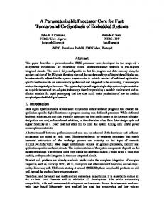
Fig. 1.
f1
regFlags
wPorts
I/O
I/O
demux
f0 BUnit
Output Registers
o0
o1 regO
r0 r1 r2 r3 r4 r5 r6 r7 r8 r9 r10 r11 r12 r13 r14 r15
Instruction Decoder
op0 op1
General processor array and processing element structure.
Avispa, Moustique, and Bresca IP-Cores (Intellectual Property Cores) from Silicon Hive [8]. Other examples are D-Fabrix from Elixent [9], the Dynamically Reconfigurable Processor (DRP) from NEC [10], or QuickSilver Technology’s Adaptive Computing Machine [11]. Existing fine-grained and coarsegrained architectures both lack programmability as a result of paradigms, which are very different from the von Neumann’s. Therefore our concept which we call weak programmability is to allow a limited, simple, and parameterizable instruction set for each processing element of the processor array. Several levels of parallelism are utilized in coarse-grained architectures. Instruction level parallelism is usually accomplished with the help of the VLIW architecture, where the functional units of a single processing element are executing instructions in parallel. The next hierarchical level of parallelism consists of different parallel working processing elements. Potentially, even higher levels are possible, like multiple coarse-grained systems integrated in a high-level array. As an example the multi-core streaming arrays from Silicon Hive can be mentioned. Since the interconnect scheme can significantly affect the type of algorithms running efficiently on the given architecture, it constitutes another interesting research subject. To the best of our knowledge only few coarse-grained architectures exist, e.g. [7], [10] which provide dynamically reconfigurable interconnect topologies. However the possibilities of these architectures are quite restricted. With the help of dynamically reconfigurable interconnect schemes a substantial gain in flexibility can be achieved. For this purpose, we developed a generic concept of an interconnect wrapper module. It allows for dynamic reconfiguration of the interconnect scheme in
coarse-grained architectures. III. A RCHITECTURE D ESCRIPTION The basic building blocks in our architecture, which we introduced in [12], are so-called weakly programmable processing elements (WPPEs), see Fig. 1. They are called weakly programmable because of the limited instruction memory in each processing element and the optimized control overhead, which is kept as small as possible. The instruction set of a WPPE is also kept small and specific to instructions commonly needed in digital signal processing. For each single WPPE the instruction set is parameterizable at compile time. Every WPPE is encapsulated by an interconnect wrapper module which is described later. At the first level, single interconnect wrapper modules are statically connected in a grid topology to form a corresponding processor array. A second, dynamic interconnection scheme is provided by the dynamic switching capabilities of each interconnect wrapper module. All possible interconnection schemes for a given processor array are defined at compile-time by means of a set of so-called adjacency matrices (exact definition follows). A. General Structure of a WPPE Each WPPE can be parameterized at compile time to contain several functional units like adders/subtractors, multipliers, shifters, and modules for logical operations. The number of specific functional units is also parameterizable at compile time. The possibility to add functional units which implement user-defined functions, like for example a FFT (Fast Fourier Transformation) is also provided. Furthermore, a WPPE contains a parameterizable register file for data and also a parameterizable register file for control signals. The parameters of
j
N out
E out
i
W out
P in
NORTH input
NORTH output
·
·
·
·
WPPE N ...
·
W in
WPPE data input
WEST config reg.
WPPE data output
·
P out
S
Interconnect Wrapper
· ⎧ ⎪ ⎨
cij ← ⎪ ⎩
1, if ∃ a possible connection between I/O ports 0, otherwise (a) Fig. 2.
E
W
SOUTH input
EAST output EAST input
·
SOUTH config reg .
·
WPPE_IN config reg .
·
MUX
WEST input
cij
WEST output
·
...
·
MUX
·
...
·
MUX
·
...
...
·
E in
EAST config reg.
MUX
MUX
·
NORTH config reg .
·
N in
S in
S out
SOUTH output
(b)
(a) Adjacency matrix example and (b) Logical structure of the reconfigurable interconnect module.
both types of register files are for example number and width of general purpose and output registers and input FIFOs (First In First Out Buffers). For transfer of data and control signals between the different storage elements like registers and FIFOs a special data transfer unit is used. B. Multiway Branch Unit For VLIW architectures multiway branch units are very often used [13]. Since a WPPE has a VLIW architecture this approach was also chosen here. With the help of a parameterizable number of branch flags a multiplexer for the selection of several branch target addresses is controlled. As a branch flag any control signal from the register file for control signals, input control signals or any status flag from any functional unit can be chosen. The different branch target addresses are given in the corresponding branch instruction. With the help of this concept n branch flags are analyzed in parallel and a total of 2n different branch target addresses can be given by only one branch instruction per cycle. C. Dynamically Reconfigurable Interconnect Wrapper An interconnect wrapper encapsulates the corresponding weakly programmable processing element and is used to describe and parameterize capabilities of switch networks. Different topologies between the single WPPEs in a weakly programmable processor array like torus, 4D hypercube, and others can be implemented and changed dynamically. To define all possible interconnect topologies, an adjacency matrix is given for each interconnect wrapper in the array at compile time. The structure of the adjacency matrix is exemplarily shown in Fig. 2(a). All input and output signals in the four directions N (north), E (east), S (south), and W (west) of the interconnect wrapper, as well as input P in and output signals P out of the encapsulated WPPE are organized in a
matrix form. The input signals of the interconnect wrapper and the output signals of the encapsulated WPPE build the rows of the corresponding adjacency matrix, and the output signals of the interconnect wrapper and the input signals of the encapsulated WPPE build the columns of the adjacency matrix. Two input and output signals in each direction of the interconnect wrapper are assumed, and two input and output ports in the encapsulated WPPE for the corresponding example interconnect wrapper and the adjacency matrix in Fig. 2(a). If an arbitrary input i and output signal j have to be connected, the variable cij in Fig. 2(a) is set to 1. Otherwise it is set to 0. If many input signals are allowed to drive a single output signal a multiplexer with an appropriate number of input signals is generated. The inputs of this multiplexer are connected to the corresponding input signals and the output to the corresponding output signal. The logical structure of an interconnect wrapper module is schematically shown in Fig. 2(b). The select signals for such generated multiplexers are stored in configuration registers and can therefore be changed dynamically. By changing the values of the configuration registers in an interconnect wrapper component different interconnect topologies can be implemented and changed at run-time. The number and width of the input and output signals of the interconnect wrapper component might be different. This is configured at compile time. D. Weakly Programmable Processor Array The interconnect wrapper components of each weakly programmable processing element is connected in a regular grid topology to form a weakly programmable processor array. Two levels of connections can be specified. The regular static connections between the single interconnect wrapper components build the first level. The second dynamic level is the current interconnect topology which is defined by the
Column: 2 1 0
groups of processing elements in an array. This scheme is explained in the following in detail.
Vertical Mask Register (V) Bit # 2
Bit # 1
Bit # 0
ICN Wrapper
ICN Wrapper
ICN Wrapper
Bit # 1
Multicast Signature: H: 1 1 0
Bit # 0
Horizontal Mask Register (H)
Bit # 2
Row: 0 1 2
ICN Wrapper
ICN Wrapper
ICN Wrapper
ICN Wrapper
ICN Wrapper
ICN Wrapper
V: 0 1 1
Multicast Signature: H: 0 0 1
Configuration Bit
V: 1 1 1
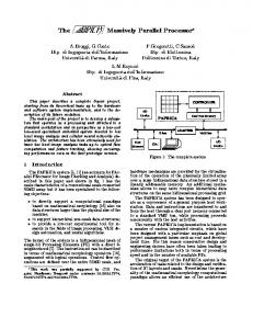
Fig. 3. Multicast configuration of the single processing elements and their interconnect modules.
values of the configuration registers. By means of the first static level of interconnect signals the problems in placing and routing of WPPEs in an array are reduced, see [4]. With the help of the second level different interconnect schemes can be changed dynamically. 1) Reconfiguration: To achieve dynamic reconfigurability of VLIW programs and the interconnect structure each WPPE has a small configuration loader component. A configuration loader is controlled by a finite state machine. Additionally, there is a global configuration controller and global memory for storage of different configurations on the WPPA level. The global configuration controller is connected to an external control unit. This can be for example an embedded processor core in a SoC (System-on-a-Chip) design. In a configuration or reconfiguration phase the global configuration controller reads the current configuration from the global configuration memory and puts the data on a global configuration data bus. The width of the global configuration memory and the configuration data bus are parameterizable at compile time. They may be different from the width of local VLIW instruction memories and the width of configuration registers in the single WPPEs and interconnect wrapper components. The local configuration loader modules in WPPEs which have to be configured run synchronously with the global configuration controller and write the received configuration words to the respective storage elements. To achieve scalability of weakly programmable processor arrays a multicast scheme was chosen. Since a global bus for reconfiguration data is used, it is important to be able also to configure and reconfigure parts of a big processor array, like for example an array of the size 10 × 10 with 100 processing elements or bigger. Otherwise a problem with the bus driver strength can arise. With the help of multicast bits in special registers it is possible to address single processing elements as well as
2) Multicast Reconfiguration Scheme: For the configuration and reconfiguration of a WPPA a multicast scheme called RoMultiC (Row Multicast Configuration) was chosen [14]. This method also allows for partial reconfiguration of a weakly programmable processor array. There is a corresponding multicast bit for each row and each column in a two-dimensional processor array. Every interconnect wrapper in the processor array is connected to one horizontal and one vertical multicast bit, see Fig. 3. If a multicast bit is set the corresponding row or column in the array is selected. Afterwards those WPPEs will be configured which have both the vertical and horizontal multicast bits set. The single multicast bits are grouped into two multicast registers: A vertical mask register for the columns of the array and a horizontal mask register for the rows of the array. Both mask registers are located in the global configuration controller and are accessible from an external control unit. For the tuple of two mask register values we use the term multicast signature. A multicast signature uniquely identifies a group of weakly programmable processing elements. This includes the case of a single processing element as well as processor array as a whole. To use the advantages of this reconfiguration scheme one could partition a given processor array e.g. in two rectangular parts each part running a different application. Then the first part could be reconfigured while an application is still running on the second part. 3) Reconfiguration Data: The global configuration memory contains the different configurations, i.e. VLIW programs and interconnect schemes. A VLIW program and an interconnect scheme are grouped to build one configuration type. Since configuration memory consumes logic resources it has to be as small as possible. Therefore in a WPPA a possibility is given to address the VLIW program configuration and the interconnect scheme separately. The width of the global configuration memory is parameterizable at compile time. It is independent of the width of the VLIW memories in the single processing elements of the array, since they all can be different on their part. This helps to control the reconfiguration time of the processor array, its scalability and flexibility. If a small width for the configuration memory is chosen, multiple configuration words have to be read to construct a single VLIW instruction. On the other side, a very wide global configuration data bus consumes more power and chip area. Therefore a tradeoff between the scalability and configuration speed has to be made. A higher flexibility can be achieved if the VLIW memories and configuration registers for the interconnect scheme can be configured separately. If for a new application the current interconnect scheme has to be changed but the programs may stay the same, only the much smaller interconnect data has to be configured. This approach corresponds to the differential reconfiguration of the processor array.
TABLE I E XCERPT FROM THE STATIC PARAMETER LIST OF A WPPE. Name
Meaning
x y u v w n m r γ φ a d f δ
Number of adder modules Number of multiplier modules Number of logic modules Number of shift modules Number of data transfer units Register operand width [bit] Immediate operand width [bit] Register address width [bit] Number of general purpose registers Number of input FIFOs VLIW memory address width [bit] VLIW memory width [bit] Number of branch flags configuration bus width [bit]
TABLE II E XCERPT FROM THE STATIC PARAMETER LIST OF A WPPA. Name
Meaning
N M wppe gen[ N ][ M ] adj mtx[ N ][ M ]
#WPPEs in vertical direction #WPPEs in horizontal direction Static parameters for each WPPE Adjacency matrix for each WPPE
IV. C ONFIGURABLE PARAMETERS A general taxonomy of configurable parameters is already given in [1]. According to this we distinguish between static and dynamic parameters. Definition 4.1: (Static Parameters). A static parameter determines the precise hardware architecture. It has to be set at compile time of the HDL code/before hardware fabrication. Often generic variables are used to represent static parameters in the HDL code. A parameterized number of hardware instances, e.g. number of general purpose registers or buffers, can also be considered as a static parameter. Definition 4.2: (Dynamic Parameters) A dynamic parameter can be changed dynamically at run-time of the fabricated hardware. It changes such characteristics as transmission rate, alternative interconnect topology, etc. It might be set by software or other hardware modules. Dynamic parameters can further be coarse-grained or finegrained. Some of the static parameters for a single processing element are given in Table I and some of the static parameters for the whole processor array in Table II. For each processor element a total of 32 static parameters can be specified. These 32 parameters can be different for different processor elements in the array. Thus, heterogeneous processor arrays can also be implemented. Each interconnect wrapper component can be considered as a coarse-grained dynamic parameter. To allow for a design space exploration technology-independent analytical hardware cost models for each processor element component were derived. In Table III hardware costs for basic hardware elements
TABLE III H ARDWARE COST OF THE BASIC COMPONENTS . Component
Name
Cost
MUX 2 1
CInv (n) Cand (n), Cor (n) Cxor (n) Cmux2 (n)
1n 2n 4n 3n
F LIP -F LOP RAM -C ELL
Cf f (n) Crcell (n)
8n 2n
NOT AND , OR XOR
1
in dependency of the operand width n are given, normalized to the cost of an inverter, see [15]. As an example we consider the derivation of the analytical hardware cost model for an interconnect wrapper component. The overall hardware cost of an interconnect wrapper module can be divided into • Cicn CFG (A): Hardware cost of configuration registers as a function of a specific adjacency matrix A. • Cicn MUX (A): Hardware cost of internal multiplexer modules as a function of a specific adjacency matrix A. For the interconnect wrapper component we can estimate the overall hardware cost as: Cicn (A) = Cicn CFG (A) + Cicn MUX (A)
(1)
The number of driver signals for a given output signal, driver signals vector �t, can be obtained after the multiplication of the transposed adjacency matrix AT with an unit vector �e: �t = AT · �e
(2)
To obtain the widths of the correspondent select signals of the multiplexer modules we take the discrete logarithm of �t: ⎞ ⎛ ⎞ ⎛ s0 �log2 (t0 )� ⎜ s1 ⎟ ⎜ �log2 (t1 )� ⎟ ⎟ ⎜ ⎟ ⎜ (3) �s := ⎜ . ⎟ = ⎜ ⎟ .. . ⎠ ⎝ . ⎠ ⎝ . �log2 (tl−1 )� sl−1 In the special case of 0 as argument, we set log2 (0) := 0. Now we define a metric as follows: ⎛ ⎞ a0 l−1 ⎜ a1 ⎟ � ⎜ ⎟ (4) ai , �a = ⎜ . ⎟ | �a | := ⎝ .. ⎠ i=0
al−1
For the minimum hardware cost of the configuration registers we get min min Cicn s ) = Cf f (| �s |) CFG (A) = Cicn CFG (�
(5)
Each of the configuration registers will generally have a different width and the resulting hardware cost for the configuration register file as a whole will be minimal. For several reasons it could sometimes be favorable to use registers of the same width for all configuration signals. Then the maximum width κ of all select signals is chosen: κ := max{s0 , s1 , . . . , sl−1 }
(6)
icn_MUX 89%
The hardware cost of such a configuration register file amounts to (7) Cicn CFG (A) ≤ l · Cf f (κ) Depending on the synthesis tool additional logic optimization could be performed which we do not consider yet. Therefore we use ≤ in Eq. (7). The case of equality is given when all components of the select signal vector �s are identical and all output signals of the interconnect wrapper and input signals of the internal processor element are connected to the output of a corresponding multiplexer: l−1 ∀i,j=0; i�=j : si = sj , si �= 0, sj �= 0
To specify the amount of Cicn MUX (A) we additionally introduce a vector for the different widths of the interconnect wrapper output signals and processor element input signals (in the same order as they appear within the corresponding adjacency matrix A): ⎛ ⎞ w0 ⎜ w1 ⎟ ⎜ ⎟ w � := ⎜ . ⎟ (8) ⎝ .. ⎠ wl−1 Now the hardware cost equation for the internal multiplexer modules of an interconnect wrapper can be specified � ≤ Cicn MUX (A) = Cicn MUX (�t, w)
l−1 � j=0
Cmuxtj (wj ) , 1
with Cmux11 (wj ) := Cconnection (wj ) and
(9)
Cmux01 (wj ) := 0 Equation (9) assumes that all driver signals for the given output signal have the same width wj as the given output signal. This might be true in particular cases, but in general all driver signals may have different widths not equal to the width of the driven output signal. This is the reason we use ≤ in Eq. (9). Cconnection (wj ) stands for the routing/area cost of a signal of the width wj . However, we do not consider such cost in our hardware cost estimations yet and it can be therefore be set to 0. Cmuxtj denotes the cost of a tj to 1 multiplexer in our 1 notation. Thus, for each interconnect wrapper module in the processor array the hardware cost can be estimated with the help of the following inequality: �) ≤ Cicn (A) = Cicn (�s, �t, w ≤ l · Cf f (κ) +
l−1 � j=0
Cmuxtj (wj )
(10)
1
V. C ASE S TUDY A highly parameterizable template was written in VHDL (Very High Speed Hardware Description Language) for the generation of weakly programmable processor arrays. An example 4×4 processor array was instantiated and tested on a Xilinx Virtex-II Pro TM xc2vp100 FPGA. To reduce synthesis and mapping time, a very simple configuration was chosen for all processing elements in the array. Each WPPE was
icn_MUX 85%
icn_CFG 15%
icn_CFG 11%
(a)
(b)
Fig. 4. (a) Theoretical hardware cost ratio for the case study interconnect wrapper and (b) Synthesis result.
configured to contain two adder modules and one module for the transfer of control signals. Data path width was chosen to be 16 bit. First a simple adjacency matrix Acs was chosen to compare the theoretically estimated hardware cost from Eq. (10) with synthesis results: ⎞ ⎛ 0 0 0 0 0 0 0 0 1 0 ⎜ 0 0 0 0 0 0 0 0 0 1 ⎟ ⎟ ⎜ ⎜ 0 0 0 0 0 0 0 0 1 0 ⎟ ⎟ ⎜ ⎜ 0 0 0 0 0 0 0 0 0 1 ⎟ ⎜ ⎟ ⎜ 1 0 0 0 0 0 0 0 1 0 ⎟ (11) Acs = ⎜ ⎟ ⎜ 0 1 0 0 0 0 0 0 0 1 ⎟ ⎜ ⎟ ⎜ 0 0 0 0 0 0 0 0 1 0 ⎟ ⎜ ⎟ ⎜ 0 0 0 0 0 0 0 0 0 1 ⎟ ⎝ 1 0 1 0 1 0 1 0 0 0 ⎠ 0 1 0 1 0 1 0 1 0 0 For the adjacency matrix Acs a configuration of two input and output signals for each direction (North, East, South, West) and two input and output ports for the corresponding processing element was assumed. The output ports of the corresponding processing element are connected to all output ports of the interconnect wrapper component and all input signals from the input ports of the interconnect wrapper component can be connected to the input ports of the corresponding processing element. Thus, a mesh interconnect architecture can be realized with Acs , for example. The estimated relation between hardware costs of the different parts of the interconnect wrapper as well as synthesis results are shown in Fig. 4. The orders of magnitude between different parts are quite accurate. This indicates that the comparison of different configurations in a design space exploration is accurate enough to take the right calculations for searching cost-optimal architectures. Furthermore, two different interconnection schemes (with other adjacency matrices) were implemented, see Table V and VI for parameter values used. The logical interconnection scheme for the 4D hypercube topology is depicted in Fig. 5(a) and for the butterfly fat tree (BFT)-like topology in Fig. 5(b). The results are shown in Table IV. It can be seen from the synthesis results, that starting from the basic mesh interconnection scheme additional interconnection configurations can be added at relative little hardware cost of roughly 2% in the case of the 4D hypercube topology. In the case of the 4D
I/O
I/O
I/O
ICN Wrapper
ICN Wrapper
ICN Wrapper
ICN Wrapper
ICN Wrapper
ICN Wrapper
ICN Wrapper
ICN Wrapper
ICN Wrapper
ICN Wrapper
ICN Wrapper
ICN Wrapper
ICN Wrapper
ICN Wrapper
ICN Wrapper
ICN Wrapper
ICN Wrapper
ICN Wrapper
ICN Wrapper
ICN Wrapper
ICN Wrapper
ICN Wrapper
ICN Wrapper
ICN Wrapper
ICN Wrapper
ICN Wrapper
ICN Wrapper
I/O
I/O I/O
I/O
I/O
ICN Wrapper
I/O
ICN Wrapper I/O
ICN Wrapper
I/O
ICN Wrapper
I/O
ICN Wrapper
I/O
I/O
(a) Fig. 5.
I/O
I/O
(b)
(a) 4D Hypercube interconnection scheme and (b) BFT-like interconnection scheme in a 4×4 array.
TABLE IV S YNTHESIS RESULTS FOR DIFFERENT INTERCONNECTION NETWORKS IN A 4×4 PROCESSOR ARRAY FOR A X ILINX xc2vp100 FPGA.
Equivalent Gates MUX 4 1 (16) MUX 8 1 (16) Logic LUT Route-Through LUT Memory LUT FPGA Resources
Mesh
4D Hypercube
4D Hypercube & Mesh
BFT-like & 4D Hypercube
859482 32 0 30287 302 4768 50%
865941 32 0 31724 244 4768 51%
880125 33 0 33296 167 4768 52%
875412 37 7 32883 140 4768 52%
hypercube with the additional butterfly fat tree topology the hardware cost amounts to roughly 1%. The configuration stream size and configuration times for a program consisting of four VLIW instructions in each WPPE can be seen in Table VII. In the best case all WPPEs in the array can be programmed with the same program and with the help of the multicast configuration this program has to be transferred only once over the 32 bit wide configuration bus. The transmission is controlled by a finite state machine. For this reason there are 5 setup and 1 end cycle for the transmission of one program. Therefore (4 × 3 + 6) cycles are needed for the transmission of our VLIW program consisting of four 79 bit wide VLIW instructions. In the worst case each WPPE in the array has a different program an has to be programmed separately. In Table VIII configuration stream size and configuration time for one of two possible interconnect schemes, in this case 4D Hypercube or Mesh, is shown. On the whole 2.88 µs + 130 ns = 3.01 µs are needed in worst case to configure the programs and the interconnect scheme of our 4×4 array. In case of fine-grained architectures this is approximately the time needed to configure a single
look-up table for Xilinx Virtex II FPGAs. The assumption for a program to consist only of four VLIW instructions is realistic, since different digital filter algorithms, like for example edge detection, can already be implemented with programs of that size. A. Results The synthesis results indicate that a significantly higher hardware flexibility grade, two different dynamically reconfigurable interconnect topologies in our case, can be achieved with a relatively small hardware overhead. Since the physical interconnect topology often gives a substantial gain in execution time for corresponding algorithms, the additional flexibility allows us to implement more different applications on the single reconfigurable coarse-grained architecture. With the help of the technology-independent analytical hardware cost models an automatic design space exploration could be applied to find an appropriate hardware architecture for the given algorithm class, like for example multimedia processing of wireless applications.
TABLE V E XCERPT FROM THE STATIC PARAMETER VALUES OF A CASE STUDY WPPE. Parameter
Value
Number of adder modules Number of multiplier modules Number of logic modules Number of shift modules Number of data transfer units Register operand width [bit] Immediate operand width [bit] Register address width [bit] Number of general purpose registers Number of input FIFOs VLIW memory address width [bit] VLIW memory width [bit] Number of VLIW instructions in a WPPE Number of branch flags Configuration bus width [bit]
2 0 0 0 0 16 5 4 8 6 8 79 4 2 32
TABLE VI E XCERPT FROM THE STATIC PARAMETER VALUES OF A CASE STUDY WPPA. Parameter
Value
#WPPEs in vertical direction #WPPEs in horizontal direction Static parameters for each WPPE Adjacency matrix for each WPPE
4 4 wppe gen[ 4 ][ 4 ] adj mtx[ 4 ][ 4 ]
VI. C ONCLUSIONS AND F UTURE W ORK A new class of highly parameterizable parallel embedded processor architectures called weakly programmable processor arrays was discussed, as well as a novel approach for dynamically reconfigurable interconnection schemes for coarse-grained reconfigurable architectures. Furthermore, a classification of architectural parameters was made. For our architecture we developed high-level technology-independent hardware cost models, see also [16]. On the basis of such abstract hardware cost models and mapping methodology we want to perform automatic design space explorations for weakly programmable processor arrays. Besides this architectural research we are currently working on retargetable compilation techniques. A preliminary overview of how to match architectural parameters and mapping methodology is given in [17]. ACKNOWLEDGMENT This project is supported in part by the German Science Foundation (DFG) in project under contract TE 163/13-1. R EFERENCES [1] T. D. Givargis and F. Vahid, “Parameterized System Design,” in CODES ’00: Proceedings of the eighth international workshop on Hardware/software codesign. New York, NY, USA: ACM Press, 2000, pp. 98–102.
TABLE VII E XAMPLES OF RECONFIGURATION STREAM SIZES AND RECONFIGURATION TIMES FOR A PROGRAM OF 4 VLIW WORDS IN THE CASE STUDY WPPA. Best Case
Worst Case
18 10 Byte 0.18 µs
288 158 Byte 2.88 µs
Number of cycles @32 bit config. bus Configuration stream size Configuration time @100 MHz
TABLE VIII E XAMPLES FOR THE RECONFIGURATION STREAM SIZES AND RECONFIGURATION TIMES FOR THE 4D Hypercube & Mesh INTERCONNECT SCHEMES IN THE CASE STUDY WPPA. Value Number of cycles @32 bit configuration bus Configuration stream size Configuration time @100 MHz
13 (1×read, 12×write) 12 Bit (12 × mux21 ) 130 ns
[2] T. J. Todman, S. J. E. Wilton, O. Mencer, W. Luk, G. A. Constantinides, and P. Y. K. Cheung, “Reconfigurable Computing: Architectures and Design Methods,” in IEE ’05: IEE Proceedings - Computers and Digital Techniques, vol. 152, 2005, pp. 193–207. [3] A. Singh and M. Marek-Sadowska, “FPGA Interconnect Planning,” in SLIP ’02: Proceedings of the 2002 International Workshop on Systemlevel Interconnect Prediction. New York, NY, USA: ACM Press, 2002, pp. 23–30. [4] R. Hartenstein, “A Decade of Reconfigurable Computing: A Visionary Retrospective,” in DATE’01: Proceedings of Design Automation and Test in Europe, Mar. 2001, pp. 642–649. [5] M. B. Taylor et al., “The Raw Microprocessor: A Computational Fabric for Software Circuits and General-Purpose Programs,” IEEE Micro, vol. 22, no. 2, pp. 25–35, Mar. 2002. [6] P. Schaumont, I. Verbauwhede, K. Keutzer, and M. Sarrafzadeh, “A Quick Safari Through the Reconfiguration Jungle,” in 38th Design Automation Conference, Las Vegas, NV, June 2001, pp. 172–177. [7] V. Baumgarte, G. Ehlers, F. May, A. N¨uckel, M. Vorbach, and M. Weinhardt, “PACT XPP – A Self-Reconfigurable Data Processing Architecture,” The Journal of Supercomputing, vol. 26, no. 2, pp. 167–184, 2003. [8] Silicon Hive, http://www.siliconhive.com. [9] Elixent Ltd., http://www.elixent.com. [10] M. Motomura, “A Dynamically Reconfigurable Processor Architecture,” in Microprocessor Forum, CA, 2002. [11] Quicksilver Technology, http://www.qstech.com. [12] D. Kissler, F. Hannig, A. Kupriyanov, and J. Teich, “A Dynamically Reconfigurable Weakly Programmable Processor Array Architecture Template,” in Proceedings of the 2nd International Workshop on Reconfigurable Communication-Centric System-on-Chips, Montpellier, France, July 2006. [13] S. M. Moon and S. D. Carson, “Generalized Multiway Branch Unit for VLIW Microprocessors,” IEEE Transactions on Parallel and Distributed Systems, vol. 6, no. 8, pp. 850–862, 1995. [14] V. Tunbunheng, M. Suzuki, and H. Amano, “RoMultiC: Fast and Simple Configuration Data Multicast Scheme for Coarse Grain Reconfigurable Devices,” in ICFPT 2005: Conference on Field - Programmable Technology, 2005, pp. 129–136. [15] S. M. M¨uller and W. J. Paul, Computer Architecture: Complexity and Correctness. Springer, 2000. [16] D. Kissler, F. Hannig, A. Kupriyanov, and J. Teich, “Hardware Cost Analysis for Weakly Programmable Processor Arrays,” in Proceedings of the IEEE International Symposium on System-on-Chip (SoC’06), Tampere, Finland, Nov. 2006. [17] H. Dutta, F. Hannig, and J. Teich, “Mapping of Nested Loop Programs onto Massively Parallel Processor Arrays with Memory and I/O Constraints,” in Proceedings of the 6th International Heinz Nixdorf Symposium, New Trends in Parallel & Distributed Computing, ser. HNIVerlagsschriftenreihe, F. Meyer auf der Heide and B. Monien, Eds., vol. 181, Paderborn, Germany, Jan. 2006, pp. 97–119.