Modeling and simulation of a photovoltaic system: An advanced synthetic study* Dhaker ABBES, Gérard CHAMPENOIS, André MARTINEZ, Benoit ROBYNS
Abstract— This paper focuses on modeling and simulation of a buck converter based on a PV standalone system. This advanced synthetic study includes PV generator modeling with parameters identification, an improved P&O (Perturb and Observe) algorithm with adaptive increment step and a detailed approach of DC-DC converter modeling. A thorough method is used to determine parameters for PI current controller. The set was used to simulate a whole photovoltaic conversion chain under Matlab/Simulink environment. A special focus has been dedicated to the influence of solar irradiation variations on converter dynamic and behavior as a range of PV current 0-8 A was considered. Simulation results confirm stability, accuracy and speed response of synthesized regulator and MPPT algorithm employed. Dynamic analyses show that the more restricting control concerns low values of current (low irradiation). This work will be useful for PhD students and researchers who need an effective and straightforward way to model and simulate photovoltaic systems. I. INTRODUCTION A photovoltaic (PV) system directly converts sunlight into electricity. Basic device of a PV system is the PV cell. Cells are grouped to form panels or arrays. The voltage and current available at output PV device may directly feed small loads such as lighting systems and DC motors. More sophisticated applications require electronic converters to process electricity from PV device. These converters may be used to regulate the voltage and current at the load, to control the power flow in grid-connected systems, and mainly to track the maximum power point (MPP) of the device [1]. This paper focus on modeling and simulation of a buck converter based on a PV standalone system. In order to study such a system, we need to know how to model the PV device associated to the converter. PV devices present a *Research supported by Region Poitou-Charentes (Convention de recherche GERENER N° 08/RPC-R-003) and Conseil General Charente Maritime. Dhaker ABBES is with the High Engineering School of Lille (HEI-Lille), 13 Rue de Toul, Lille, France, phone: 0033328384858 e-mail:
[email protected] Gérard CHAMPENOIS is with LIAS-ENSIP, University of Poitiers, Bat. B25, 2 rue Pierre Brousse, B.P. 633, 86022 Poitiers Cedex, France, phone : 0033549453511, E-mail :
[email protected]. André MARTINEZ, is with the Engineering School of Industrial Systems (EIGSI-La Rochelle) and LERPA Research Manager, 26 rue de vaux de Foletier, 17041 La Rochelle Cedex 1, France, phone : 00 33 5 46 45 80 45 E-mail:
[email protected] Benoit ROBYNS is with the High Engineering School of Lille (HEILille) and Laboratory of Electrical Engineering and Power Electronics (L2EP), 13 Rue de Toul, Lille, France. phone: 0033328384858 e-mail:
[email protected]
nonlinear (I, V) characteristic with several parameters that need to be adjusted from experimental data of practical devices. The mathematical model of the PV device may be useful for investigation of dynamic analysis of converters and MPP tracking (MPPT) algorithms, and mainly to simulate the PV system and its components using circuit simulators. Then, it is important to model converter and to design adequate proportional and integral compensators to control inputs (voltage or current or both) of the converter. All these aspects are treated in this paper and a particular emphasis is focused on the modeling and control of DC-DC converter. Control of the input voltage of DC-DC converters is frequently required in photovoltaic (PV) applications. In this special situation, unlike conventional converters, the output voltage is constant and the input voltage is variable. Converters with constant output voltage are well known. Buck, boost and other topologies have been employed in PV applications where input is controlled instead of output. In most of works and investigations, power tracking methods and other subjects regarding the PV system control are studied, but a little attention is given to the converter [2]. References [3-5] are showing systems where a PV array and a battery are interfaced with a buck converter (output voltage of converter is essentially constant) and study power tracking algorithms to adjust the condition of the PV array in order to match desired operating point. Few authors have investigated the input control of converters with a mathematical approach. In [6], the authors present the analysis of open-loop power-stage dynamics relevant to currentmode control for a boost pulse width-modulated (PWM) DC-DC converter operating in Continuous-Conduction Mode (CCM). In [7], boost converter with input control for PV systems is analyzed. In [8], there is a study of the buck converter with controlled input used in a PV system. Finally, Kislovski [9] makes considerations about the dynamic analysis of the buck converter employed in a battery charging system. Although many papers bring information and even experimental results with buck-based systems, many questions still remain unanswered. These questions consider dynamic behavior of the buck converter (especially for irradiation) with constant output voltage and the design of proportional and integral compensators to control the input current of the converter. So, in this paper, detailed approaches for modeling DC-DC converter as well as a method for determining parameters of PI controller are discussed. Detailed and specific calculations are applied and a study of the influence of solar irradiation variations on converter dynamic and behavior is conducted. A range of PV current 0-8 A was considered. The paper is organized as follows: Section II concerns PV generator modeling. Model is described and photovoltaic panel parameters are identified using a lever iterative algorithm. Then, in section III, an improved P&O (Perturb and Observe) algorithm with adaptive increment step is detailed.
Finally, in the remaining sections, we are interested in the simulation of the complete system under Matlab / Simulink and in the synthesis of DC-DC converter PI current regulator parameters. An analysis of converter behavior and influence of solar irradiation variations on its dynamics is presented then simulation results are shown.
II. PV GENERATOR MODELING A. Model Description In the literature, a photovoltaic cell is often depicted as a current generator with a behavior equivalent to a current source shunted by a diode. To take into account real phenomena, model is completed by two resistors in parallel and series Rs and Rp as shown in figure 1 [1].
is the rated short-circuit current under nominal conditions of temperature and irradiation (under and ). The saturation current also depends on the temperature according to the following expression: [
(
)]
(4)
with: Eg is energy bandgap of the semiconductor, polycrystalline silicon panels [1] [10]. is the nominal saturation current given by: (
for
(5)
)
where: corresponds to nominal voltage vacuum and to coefficient of variation of the voltage as a function of temperature.
B. Photovoltaic panel parameters identification In our case, simulated panels are "Sharp ND-240QCJ Poly" with a peek power of 240Wp. Properties of solar panel, according to the technical specification sheet, are shown table I. TABLE I.
ELECTRICAL CHARACTERISTICS OF SHARP ND-240QCJ POLY (240WC), SOLAR PANEL Electrical characteristics of the ND-240 Poly Pmax Isc Voc Imp Vmp
Figure 1. PV generator model with a single diode and two resistors
Current Ipv generated by the panel is expressed as a function of Rs and Rp resistors, voltage and currents and , as follows: [ ( ) ] (1)
240 Wc 8.75 A 37.5 V 8.19 A 29.3 V 53 x 10-5 A/K -36 x 10-3 V/K
KI KV
With: : photovoltaic current due to irradiation. If the panel is composed of Np cells connected in parallel, then where is the saturation current for a single cell, : saturation current of the PV panel. where is the current of a single cell and the number of cells in parallel, : thermal potential of the panel.
,
is number
of cells in series, K: Boltzmann constant [ ], q charge of an electron [ ] and T temperature of the p-n junction in Kelvin degree [°K]. T is assumed equal to the ambient temperature. a: ideal constant of the diode, assumed equal to 1 in our case. Vpv: voltage across the panel. The photovoltaic current is linearly dependent on the irradiance (G) and is also influenced by the temperature T according to the following equation:
(
)
(2)
is the photovoltaic current generated at nominal conditions ( = 298.15 K and 1000 W/m²), and coefficient of variation of current as a function of temperature. (3)
Unfortunately, not all the parameters are given in the data sheet. The values for Rs and Rp are missing and have to be found in another way. When taking a look at the formula for the maximum power output, we see that these parameters are easily extractable. {
{
[
(
[
)
]
]
(6)
}
}
(7)
Imp and Vmp are respectively current and voltage of photovoltaic panel at maximum power point. is maximum power deduced via model identification procedure and is the experimental maximum power indicated by the panel manufacturer under nominal conditions. To find Rp value, we have to find a value of Rs so that is equal to ( . This is possible with an iterative algorithm. For this purpose, we can use the procedure described by MG Villalva and al. [1] and represented by the flowchart in Figure 2.
Figure 4. Evolution of the maximum power of the photovoltaic panel "Sharp ND-240QCJ Poly (240Wp)" depending on the ambient temperature (Ta) and irradiance (G)
Figure 2. Iterative algorithm to find the Rs and Rp parameters
To compute this algorithm, initial values for Rs and Rp are needed. The value for Rs,ini is fixed to zero and Rp,ini is found by substituting Rs by zero in the equation (7): (8) Using the procedure, we obtain the following values for Rs and Rp:
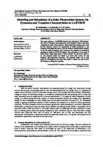
{ With these parameters we can represent the electrical characteristics (Figure 3) of the photovoltaic panel "Sharp ND-240QCJ Poly (240Wp)" and present the evolution of its maximum power as a function of ambient temperature (Ta [° C]) and the irradiance (G [W/m²]) (Figure 4). 250
Ppv [W]
200
150
It is interesting to note that after calculation of the different values of the maximum power depending on the ambient temperature Ta [°C] and irradiance G [W/m²], it is possible with a "fitting" under Matlab to have a polynomial model of the panel as follows: (9) In this paper, we are focusing on parameters to consider for the simulation. More generally, this model could be useful to estimate photovoltaic production or could be employed for the design of a simple method of Maximum Power Point Tracking.
III. DESCRIPTION OF MAXIMUM POWER POINT TRACKING (MPPT) ALGORITHM In the literature, there are different types of MPPT algorithms for photovoltaic systems [11]. In our case, an improved P&O algorithm is chosen with adaptive increment step [12]. Fundamental principle of this method is increment step variation to converge faster towards optimal point (MPP) while reducing oscillations around. Indeed, in order to quickly converge, increment step C is reduced or adapted from a region to another: C = 0.01 in "S" region and 0.001 in "r" region (Figure 5). MPPT algorithm is shown Figure 6.
100
50
0
0
5
10
15
20 Vpv [V]
25
30
35
40
Figure 3.a Evolution panel power as a function of the voltage across 9 8 7
Ipv [A]
6 5 4 3 2 1 0 0
5
10
15
20 Vpv [V]
25
30
35
40
Figure 3.b Evolution of the current generated by the photovoltaic panel as a function of the voltage across Figure 3. Characteristic curves of the "Sharp ND-240QCJ Poly (240Wp)" (G = 1000W / m², Ta = 25 ° C)
Figure 5. Principle of the P&O algorithm with an adaptive step increment [12]
The control unit consists of the MPPT algorithm and the PI regulator for the current loop as shown in Figure 8.
Figure 8. Block Diagram of the MPPT control developed in Matlab / Simulink
The parameters of the PI compensator for current loop are calculated as follows:
Figure 6. Flowchart of the improved P&O MPPT algorithm
IV. DEVELOPMENT AND SIMULATION OF A PHOTOVOLTAIC
B. Procedure for determining the parameters of the PI corrector To calculate the PI parameters for the current input use the average model of the next chopper [6]:
control, we
SYSTEM
A. System description The simulated photovoltaic system consists of four main components: • photovoltaic generator composed of two panels "Sharp ND-240QCJ Poly (240Wp)", •energy storage device (battery or accumulator) • control system (controller): here it is a step down chopper current controlled by an MPPT unit and via a PI compensator • load (assumed to be continuous in this work). The set is simulated with Matlab / Simulink / Simpower as shown in Figure 7. The parameters used are summarized in Table II. TABLE II. PARAMETERS USED FOR SIMULATION IN MATLAB / SIMULINK / SIMPOWER Parameter
Value
L C Rabt Vbat Charge Pas de simulation Fréquence PWM
3 mH 1,1 mF 0,001 48V 4,8 10-6 s 20Khz
Figure 9. Average model of the chopper in interface between the photovoltaïc panels and the battery
According to this model, there are two state variables: voltage and current with the following expressions in the formalism of Laplace (s): (
{
)
(10)
}
Our objective is to control the current acting on the duty cycle . However, we note from the two equations above that the transfer function between and is nonlinear. For this reason, we propose to express a transfer function linearized around an operating average point, considering: and {
}
(11)
Thus, variables are defined as follows: {
̃
̃
̃
̃
}
(12)
From (10) and (11), we obtain: {
̃
̃
̃
̃ ̃
̃
̃
̃
̃ ̃
̃
}
(13) ̃ negligible compared to the other Considering ̃ ̃ and ̃ terms, we obtain the following system: Figure 7. Schematic of the photovoltaic conversion chain developed in Matlab / Simulink / Simpower
{
̃ ̃
̃
̃ ̃
̃
̃
}
(14)
Due to the presence of solar panels (PV) at the entrance of the chopper, there is a link between ̃ and ̃ we must express. The optimum operating point of PV generator is normally situated on the hyperbole (zone) of equal power, that is to say . So, according to equation (12), we can write: ̃
̃
̃
Neglecting ̃
(20)
̃
(15) is chosen equal to the pole (compensation pole/zero) and with a bandwidth of 1 rad / s ; which gives :
̃ to the other terms, we have:
̃
(16)
̃
Substituting
̃ by
replacing
by
̃
into (13), eliminating
and
into (11), we can express the transfer function
between ̃ and ̃ . Considering
, we obtain :
̃
, (21)
Then
.
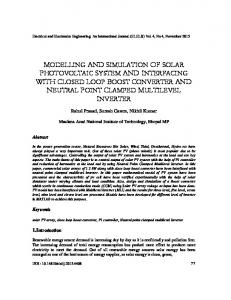
Figure 10 shows the plot of the Bode diagram for the transfer functions of open and closed loops ( and ) for ans .
(17)
̃
Then:
̃
(18)
̃
With:
;
;
√
and
√ So the transfer function between ̃ and ̃ is a system with a zero inversely proportional to (irradiation), two complex conjugate poles almost constant because little depends from irradiation, a damping factor and a gain proportional to . With the numerical application: L = 3 mH, C = 1100μF, Vbat = 48 V, Vpvo = 60 V, means
Figure 10.a Bode diagram of open and closed loops (Case
)
, we obtain:
;
;
;
. When varying
from 0 to 8A, we have always
,a
gain varying approximately between 0 and 20 and a damping coefficient that still small. Thus, the more restricting control concerns low values of current
(low irradiation).
Example: For (with a peak of ), we obtain a transfer function with poles at 440 rad/s and a damping coefficient of , which gives a resonance gain of . So to avoid resonance in closed loop, it √
is necessary to reduce the bandwidth. We choose a bandwidth of 1 rad /s. At this frequency, the transfer function can be reduced to the gain: then the transfer function with a PI regulator :
Figure 10.b Bode diagram of open and closed loops (Case
)
Figure 10. The Bode plot of the transfer functions for the open and closed loop and closed loops ( and ) for and .
becomes : (19)
V. SIMULATION AND CONTROL RESULTS Simulation results of the photovoltaic conversion chain developed in Matlab / Simulink / Simpower (figure 7) are shown below. They confirm the stability, accuracy and speed response of the synthesized regulator and used MPPT algorithm.
Finally, this paper with its quantity of information, its references and its synthetic aspect will be useful for PhD students and researchers who need an effective and straightforward way to model and simulate photovoltaic systems.
ACKNOWLEDGMENT The authors would like to thank Region Poitou-Charentes (Convention de recherche GERENER N° 08/RPC-R-003) and Conseil General Charente Maritime for their financial support.
REFERENCES Figure 11.a irradiance profile versus time used for the simulation
Figure 11.b Maximum power tracking over the time Figure 11. Simulation results of the photovoltaic system conversion chain under Matlab / Simulink
VI. CONCLUSION In this paper, an advanced synthetic study of a standalone buckbased PV system is presented. It includes: PV generator modeling and its parameters identification, an improved P&O (Perturb and Observe) algorithm with adaptive increment step, a detailed approach to the modeling of DC-DC converter and a thorough method for determining the parameters of the PI controller used for converter current control. This study has yielded some benefit results: The model presented in section II was integrated in a programmable power source to emulate two solar panels in a PV system. By calculating different values of the maximum power for various ambient temperatures Ta [°C] and irradiances G [W/m²], we have established an accurate polynomial model of the PV panel used ("Sharp ND240QCJ Poly (240Wp)"). Section IV has presented the development of converter average model and transfer functions for the input current control of the buck converter operating with duty-cycle control (current mode) and with inductor peak current control (current-programmed mode). The transfer functions reveal important dynamic characteristics of the input-controlled buck converter when it is fed by a PV array. They show that the more restricting control concerns low values of current (low irradiation). With these transfer functions it is possible to design compensators and feedback controllers for the control of the input current of the buck converter. Simulation results confirm the stability, accuracy and speed response of the synthesized regulator and used MPPT algorithm. However, these results should be experimentally validated using a PV system test bed.
[1]
M. G. Villalva, J. R. Gazoli, E. Ruppert F., “Modeling and circuitbased simulation of photovoltaic arrayes”, Brazilian Journal of Power Electronics, vol. 14, n° 1, pp. 35-45, 2009. [2] M. G. Villalva, E. Ruppert F., “ Dynamic analysis of the inputcontrolled buck converter fed by a photovoltaic array”, Revista Controle & Automação, Vol.19, n°.4, pp. 463--474, Outubro, Novembro e Dezembro 2008 [3] Koutroulis, E., Kalaitzakis, K. and Voulgaris, N., “Development of a microcontroller-based photovoltaic maximum power point tracking control system”, IEEE Trans. on Power Electronics, Vol.16, n°1,pp. 46–54, January 2001. [4] Martins, D., Weber, C. and Demonti, R., “Photovoltaic power processing with high efficiency using maximum power ratio technique”, in Proc. 28th IEEE IECON, v. 2, 2002, pp. 1079–1082. [5] Salas, V., Manzanas, M., Lazaro, A., Barrado, A. and Olias, E., “The control strategies for photovoltaic regulators applied to stand-alone systems”, Proc. 28th IEEE IECON, v. 4, 2002, pp. 3274–3279. [6] B. Bryant, M. K. Kazimierczuk, “Open-loop power-stage transfer functions relevant to current-mode control of boost PWM converter operating in CCM,” IEEE Transactions on Circuits and Systems I, Vol. 52, n° 10, pp. 2158-2164, 2005. [7] Xiao,W., Dunford,W., Palmer, P. and Capel, A. “Regulation of photovoltaic voltage”, IEEE Trans. on Industrial Electronics, Vol. 54, n° 10, pp. 1365–1374, 2007. [8] Cho, Y.-J., Cho, B., “A digital controlled solar array regulator employing the charge control”, in Proc. 32nd IECEC, v. 4, 1997, pp. 2222–2227. [9] Kislovski, A. S., “Dynamic behavior of a constant frequency buck converter power cell in a photovoltaic battery charger with a maximum power tracker”, in Proc. 5th IEEE APEC, 1990. [10] W. De Soto, S. Klein, W. Beckman, “Improvement and validation of a model for photovoltaic array performance,” Solar Energy, vol. 80, n° 1, pp. 78-88, 2006. [11] V. Salas, E. Olías, A. Barrado et A. Lázaro, “Review of the maximum power point tracking algorithms stand-alone photovoltaic systems,” Solar Energy Materials and Solar Cells, vol. 90, n° 11, pp. 1555-1578, 2006. [12] T. A. Singo, A. Martinez, S. Saadate, “Designing and Experimenting an Auto-Adaptive Controller for Stand-Alone Photovoltaic System with Hybrid Storage”, International Review of Electrical Engineering IREE Journal, Vol. 7. N°1, pp. 3391-3400, 2012.