Modeling and Solution of a Complex University Course Timetabling Problem Keith Murray1 , Tom´aˇs M¨ uller1 , and Hana Rudov´a2 1
Space Management and Academic Scheduling, Purdue University 400 Centennial Mall Drive, West Lafayette, IN 47907-2016, USA
[email protected] [email protected] 2 Faculty of Informatics, Masaryk University Botanick´ a 68a, Brno 602 00, Czech Republic
[email protected]
Abstract. The modeling and solution approaches being used to automate construction of course timetables at a large university are discussed. A course structure model is presented that allows this complex real-world problem to be described using a classical formulation. The problem is then tackled utilizing a course timetabling solver model that transforms it into a constraint satisfaction and optimization problem. The tiered structure of this approach provides flexibility that is helpful in solving the multiple subproblems that arise from decomposition of the university-wide problem. A production system has been partially implemented and results of early use are presented. Practical issues raised during the implementation of the automated timetabling system are also discussed.
1
Introduction
Timetabling is a widely studied area and many potentially useful algorithms have been offered for solving the university course timetabling problem, as evidenced by several recent surveys [7, 19, 16]. Unfortunately, much of the work in this area has been conducted using artificial data sets or based on actual problems that have been greatly simplified. Methods developed have also rarely been extended to the solution of actual university problems of any large scale. McCollum offers a good review of this situation in [11]. The major differences between many of the problems studied and their reallife counterparts are the additional complexity imposed by course structures, the variety of constraints imposed, and the distributed responsibility for information needed to solve such problems at a university-wide level. University timetabling problems may also involve the solution of multiple subproblems with very different characteristics. In practice, therefore, the solution process should not be specifically tailored to a single problem type. The work described here has been motivated by the need to create and modify course timetables at Purdue University that better meet student course demand
and allow students to be assigned to the constituent course sections in a way that minimizes conflicts. Purdue is a large (39,000 students) public university with a broad spectrum of programs at the undergraduate and graduate levels. In a typical term there are 9,000 classes offered using 570 teaching spaces. Approximately 259,000 individual student class requests must be satisfied. The complete university timetabling problem is decomposed into a series of subproblems to be solved at the academic department level, where the resources required to provide instruction are controlled. Several other special problems, where shared resources or student interactions are of critical importance, are solved institution wide. A major consideration in designing the system has been supporting distributed construction of departmental timetables while providing central coordination of the overall problem. This reflects the distributed management of instructional resources across multiple departments at the University. The general definition of the university-wide timetabling problem described in this paper is similar to the problem studied by Carter [6] at the University of Waterloo, and the influence of that work can be seen here, though the solution methods used differ significantly. It is hoped that the results of the present work will, likewise, be beneficial to other institutions seeking to improve their ability to construct course timetables for their students. This paper discusses the approach used for modeling and solving the additional complexities involved in developing automated solution techniques for a real-life course timetabling problem on the scale of a large university. Although a specific example is discussed, many of the methods used should be applicable to modeling and solving other complex problems. The complexity of the university course timetabling problem studied here has been broken down by developing a logical data model allowing all courses to be represented as hierarchical groupings of classes with additional parent– child relationships and constraints governing their placement. This allows use of one standard class-oriented problem formulation rather than having to develop different models and solution methods to work with the wide variety of ways that departments organize the instruction given in their courses. A flexible and general solution technique has been developed for solving course timetabling problems and applied to all of the departmental and special subproblem. Rather than applying multiple solution methods, each optimized around the characteristics of a specific problem, a single solution approach allows the outcomes of all of these subproblems to be easily combined into a complete solution and facilitates optimization of the sectioning of students across the complete timetable. Each of these topics will be explored in greater depth in the next three sections of this paper, followed by observations on creating a general framework that is very useful in developing a practical solver. Several practical issues faced while implementing a real-world system are then discussed, including competitive behavior among users, making changes to solutions, and managing data consistency. Some results from actual use of the system to solve departmental and campus problems are also presented. In addition, links are provided to the
problem data used in this work to promote further study by other researchers using real data instances.
2
Problem Decomposition
Timetabling is a resource allocation problem; therefore, at most universities responsibility for constructing the timetable is distributed among the academic units with the faculty, physical facilities, and other resources required for offering instruction. Providing support for this distributed responsibility is important because departmental timetablers have a much more intimate knowledge of the needs of the courses offered, the faculty who might be able to teach a particular class, and the spaces available for specialized instruction than any database that might be maintained centrally. Maintaining each department’s sense of ownership in the timetables that are produced is also an important factor in their acceptance of the solutions produced by an automated timetabling process. The process needs to be one that assists them rather than replaces them. Student degree programs may or may not consist of courses offered primarily within a single academic unit. If they do, the larger university timetabling problem may be decomposed into a series of departmental problems with little likelihood of creating class time assignment conflicts for students. A number of individual departmental or school level problems have been studied in the literature [9, 1, 5, 17]. The problem becomes more complex, however, when students attend courses from multiple academic units and the solutions are dependent upon the availability of students for the classes across multiple problems. Here the overall problem can not be easily decomposed along the lines of academic units and additional coordination is required. In the case of Purdue University, there are many large introductory courses that serve students in almost all degree programs. Since there are substantial numbers of students enrolled in more than one of these courses, they create a large dependency between the timetables of individual departments offering instruction. To deal with this, the cluster of large courses with students from many disciplines is split off as a separate problem that is solved by a central scheduling office with input from departmental timetablers. This problem is solved first, assigning times in a set of centrally managed lecture facilities, so that the results are available to all of the departmental timetablers as they solve the remainder of their problems. Most of the courses in the departmental problems primarily serve students in programs offered by that department. There are other groupings that occur however. There are several colleges where four or five departments create their timetable together because all of the departments provide courses that serve the same degree program. There are also several special problems, such as assigning classes that require shared campus computer laboratories. The ability to solve all of these different types of problems is one of the major challenges in automating the timetabling process at a large university. To better understand the effect on solution quality of decomposing the problem into multiple parts, some post timetabling experiments were run solving all
Table 1. Combined Solution Properties of Four Problems (Spring 2007)
Test case Assigned variables Time [min] Student conflicts Preferred time [%] Preferred room [%] Preferred distribution [%]
Final Run Separately Run Combined 1756.0 1756.0 ± 0.0 1756.0 ± 0.0 31.8 ± 5.9 44.1 ± 9.7 1258 907.7 ± 25.1 849.9 ± 27.4 86.2 90.6 ± 0.7 91.2 ± 1.1 82.8 83.7 ± 0.5 83.9 ± 0.4 61.0 66.4 ± 3.7 71.6 ± 3.4
of the parts together as a single problem. Although data for all departmental and other special problems at the University is not yet available, comparison of several parts addressed separately and combined as a whole gives some indication of what is lost in solution quality as a result of the decomposition. Table 1 shows a summary of several measures of solution quality3 for the large lecture problem, the central computing labs, and two different departmental problems when run separately and when combined. The same room resources were used for the separate and combined runs. As expected, there is a decrease in the number of student conflicts when all of the problems are considered together. There is also a slight improvement in the overall satisfaction of time, room, and distribution preferences. These improvements must be considered as theoretical, however, since the combined solution has not been reviewed and accepted by all of the schedule managers who have the real final say on solution quality. The column labeled final summarizes these same measures of solution quality for the actual final timetables produced by University schedule managers using this application for Spring 2007. These solutions were initially computed individually using the automated solver (see Section 4); however, some additional changes were applied manually later in the process using the solver in its interactive mode (see Section 6.2). 2.1
Interactions Between Problems
As described in the previous section, the Purdue University timetabling problem is naturally decomposed into – a centrally timetabled large lecture room problem (about 800 classes timetabled into 55 rooms with sizes up to 474 seats), – individually timetabled departmental problems (about 70 problems with 10 to 500 classes using departmental laboratory spaces and centrally managed classrooms allocated to departments based on expected class hours), 3
Average values and RMS (root-mean-square) variances between the best solutions found for 10 different runs are presented. Run time is 30 minutes for individual problems and 120 minutes for the combined problem using 2.13 GHz Pentium M, Java 1.5.0, 2GB RAM.
– and a centrally timetabled computer laboratory problem (about 450 classes timetabled into 36 rooms with 20 to 45 seats). The large lecture room problem consists of the largest classes on campus that are attended by students from multiple departments. This problem is also very dense. On average, rooms are utilized over 70% of the available time, and this rate increases with room size (utilization is over 85% for all rooms above 100 seats and about 97% for the four largest rooms having over 400 seats). Since there are many interactions between this problem and the departmental problems, the large lecture problem is solved first and the departmental problems are solved on top of this solution. On the opposite end of the spectrum, the computer laboratory problem is solved at the very end of the process, on top of the large lecture room and departmental problem solutions. It contains only small classes, most of which have many sections (laboratories are normally the smallest subparts of a course). A typical example is a course having one large lecture class for 100 students, two departmental recitations with 50 students each, and four computer laboratories of 25 students. The departmental problems are solved more or less concurrently. These problems are usually quite independent of one another, occurring in mostly different sets of rooms, with separate instructors and students. However, there are some cases with higher levels of interaction, particularly among students. In order to address these situations, a concept referred to as “committing” solutions has been introduced. Each user of the timetabling system (e.g., a departmental schedule manager) can create and store multiple solutions. At the end of the process a single solution must be selected and committed. During the commit, all conflicts between the current solution and all other solutions that have already been committed are checked and the commit is successful only when there are no hard conflicts between these solutions. Each problem being solved also automatically considers all of the previously committed solutions. This means that a room, an instructor, or a student is available at a particular time only if that time is not already occupied in a commited solution for a different problem. This approach can be beneficial, for instance, in a case where there are two or more departments with many common students. Here, the problems can be solved in an agreed upon order (the second department will solve its problem after the first department commits its solution). Moreover, if a room must be shared by two departments, a room sharing matrix can be defined, stating the times during the week that a room is available for each department to use. Finally, there is also an option to combine two or more individual problems and solve as one larger problem, considering all of the relations between the problems in real time. 2.2
Problem Characteristics
Each of the problems that the overall university timetabling problem has been decomposed into has characteristics that are different from many of the other problems. Some of the different attributes of the large lecture room problem (LLR),
computer laboratory problem (LAB) and two selected departmental problems (D1, D2) are listed in Table 2. Table 2. Characteristics of Selected Problems (Spring 2007)
Problem
LLR
D1
D2
LAB
Number of classes 804 440 69 442 1.25 3.52 1.50 4.8 Avg. number of classes per type of instruction Avg. number of hours per class 2.40 2.43 2.30 1.97 Avg. number of meetings per class 2.09 2.32 1.67 1.25 Avg. number distribution constraints per class 0.68 2.94 0.78 1.82 Number of rooms 55 25 6 36 Room sizes 40 − 474 24 − 51 14 − 48 20 − 45 Avg. room utilization [hours/week] 35.0 42.8 26.5 24.2 223.9 83.9 21.5 159.7 Average distance between rooms [m] Number of students 27881 11992 1312 8408 3.15 1.11 1.40 1.14 Avg. number of classes per student Classes with an instructor assigned [%] 69.8 33.9 60.9 13.35 Avg. number of classes per instructor 1.25 1.49 1.68 2.11
If solved independently, the large lecture room problem is the most difficult. In addition to being the largest problem in terms of number of classes, it must consider more students requesting multiple classes within the problem, rooms with a greater variation in size, very high utilization in the larger rooms, and large distances between some rooms. There are also fewer alternatives for sectioning student enrollments. The average number of classes per type of instruction offered as part the course (e.g., lecture, laboratory) is only 1.25. For departmental problems, besides the properties listed in Table 2, it is also necessary to consider that they are being built on top of the large lecture problem and that there are many teachers and students in common between them and the LLR problem. This can be an even greater complication for the computer laboratory problem, since it is being built on top of all of the other problems.
3
Modeling the University Course Timetabling Problem
Arguably, the biggest obstacle to solving actual university course timetabling problems is that the complexity can increase considerably beyond that represented in standard formulations of the problem [7, 19, 16]. As the complexity increases, it is easy to be caught in the dual bind that the problem is both more challenging to develop an effective solution approach for, and this approach is
less likely to be usable on other university timetabling problems, or even on all problems that may exist at a single institution. This complexity arises from many aspects of real-life problems. Among the most important are the structure of course offerings and the wide range of constraints that arise. As noted above, student enrollments across disciplines and shared use of resources between autonomous departments are also of concern. Other factors include the number and uniformity of the meeting times, dates, and locations over which classes need to be assigned. 3.1
Course Structure
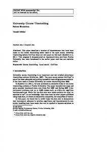
The structure of course offerings may be the most problematic. Although the problem is generally labeled “course timetabling,” in actuality it is the individual classes that make up a course which must be timetabled. In this paper, a class is defined to be a series of similar meetings for a subset of students enrolled in the course. Courses are usually composed of multiple classes that may be known as lectures, tutorials, laboratories, etc. Students normally enroll to various course offerings that are required to meet the requirements of their degree program, and most university information systems are organized around courses (known as modules in some regions) as the unit of instruction. The modeling problem becomes one of creating a logical data structure that can be used to translate all parts of the course structure, and the relationships between these parts, into a set of classes and an extended set of constraints between them. The complex real-life problem can then be solved at the class level using a standard formulation of the course timetabling problem. To incorporate all of the course structures found in the Purdue problem, a four level model was developed that breaks down each course into as many as four tiers to reflect the relationships among all of the classes that constitute it. While in a simple lecture course the class and the instructional offering are one and the same, for a large course there may be tens or hundreds of classes associated with a single instructional offering. A diagrammatic representation of the course structure model and an example showing the parts of a more complex course is shown in Figure 1. A more detailed description of each layer in this model is given in the paragraphs below. For the sake of clarity, the term instructional offering has been used in this model to distinguish the highest level of the structure from course, which is the more usual term for a series of lessons containing the subject matter to be taught. This was necessary since many universities have adopted the habit of listing the same subject matter in their course catalogs under more than one subject and course number. This boutique naming system can create quite a complication when attempting to automate timetabling since it results in many courses requiring the same times in the same rooms with the same instructors. It is also difficult under this system to know how many students are actually being taught together. The model addresses such cases by treating all course identifiers as pseudonyms and linking the courses together to form a single instructional offering. Naturally, all courses that are linked together must have
Instructional Offering Configuration Alternate Listing
Subpart Parent Child
Class
MA 100 – Calculus ENGR 101
Lecture Recitation
Lec 1 Rec1 Rec2 Rec3
Traditional
multiple offerings. . .
Lec2 Rec4 Rec5 Rec6
Computer-Aided Lecture Recitation
Lec3 Rec7 Rec8 Laboratory Lab1 Lab2
Fig. 1. Model of course structure. Example shows representation of an instructional offering with two catalog listings, two alternate configurations, and two subparts linked by a parent–child relationship.
the same structure. The alternate listing below instructional offering in Figure 1 indicates this linkage with other courses that actually meet together as part of a single instructional offering. The instructional offering is the basic organizing unit in this model. The offering is then divided into its constituent classes, which are the unique entities to be timetabled. Many courses (or instructional offerings in the model’s terminology) have multiple subparts, such as tutorials or laboratories, that are associated with a parent lecture. In some cases, the course may even be offered with different configurations of these subparts. One instructor, for example, may wish to teach the course material entirely in a lecture format whereas another may wish to devote one day per week to small discussion groups. The configuration level is included in this model to account for these types of situations. At the subpart level, the type of instruction usually takes on different characteristics. The students in the course may be divided into smaller groups for different activities and other types of facilities may be required. It may or may not be important for one group of students to be together in two or more different subparts of a course, such as wanting all students sectioned into a discussion group to also be in a laboratory together. To accommodate such needs, a parent–child relationship has been included in the model at the subpart level. If a parent–child relationship is established between two subparts, all students in a class belonging to the child subpart must also be sectioned to the appropriate parent class. Constraints are generated prohibiting an overlap in time between parent and child classes. In the GUI built for entering data, these parent–child relationships are set up much like file folders in a directory tree as indicated by
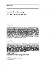
the indented subparts in Figure 1. Any attributes or preferences that apply to all classes within a subpart can be set at the subpart level. An illustration of how the structure is displayed by the interface is shown in Figure 2.
Fig. 2. Structure of classes as displayed in user interface. The configuration is displayed in the gray shaded area. Individual classes to be timetabled are listed below.
Timetabling takes place at the class level. There will typically be multiple classes associated with each subpart, especially when tutorial or laboratory sections are involved. Each class inherits attributes and preferences set on the subpart level, or these may be set for an individual class. Attributes or preferences set at the class level will override those set at higher levels. Each class must indicate the amount of time it meets, desired meeting pattern, weeks the class should meet during the term, and facility needs. Specific time, room, and room feature preferences or requirements may also be set. If an instructor is entered, preferences may also be inherited from those set on the instructor. 3.2
Constraints
The large number and variety of constraints that arise, both from the class structure and special requirements, also adds to the difficulty in finding a solution to real problems. In addition to the usual constraints specifying that an instructor
can only teach one class at a time, there can only be one class per room, and the room must accommodate class requirements, each of the departmental and special problem instances has additional hard and soft constraints that differ according to the concerns of the individual unit. This imposes a demand that the solution method must be very robust so that it can accommodate each of these different problem formulations. Each schedule manager is able to set whatever hard or soft constraints are considered necessary on the problem he/she is responsible for. These fall into the categories listed in Table 3. A consistent scale (required, strongly preferred, preferred, neutral, discouraged, strongly discouraged, prohibited) is established for setting all of these constraints. Required and prohibited indicate hard constraints. Distribution constraints may be set between individual classes or between all classes associated with an instructional offering or subpart. Managers may also override the normal hard constraint requiring one class per room by setting the number of rooms an individual class should be timetabled to.
Table 3. User Set Constraints Time: Rooms: Room Features: Class Distribution:
Meeting Time Pattern Individual Times Specify Individual Buildings/Rooms Specify User Defined Room Group Select Based on User Defined Set of Features Time Between Time Order of Classes Place Classes in Time Groups Use Same Meeting Dates/Times Spread in Time Restrict Classes Meeting at Same Time Room Sharing
As noted in the section on course modeling above, a number of additional constraints are automatically set on each problem due to the structure of the course. These require a student to be sectioned into one class for each subpart and prohibit conflicts between parent and child classes. Time assignments for all classes within a subpart are also automatically spread across all non-prohibited times. In addition, an automatic calculation of distances between rooms is performed to penalize class placements that require students or instructors to travel large distances between consecutive classes. There is also a set of constraints that seek to ensure efficient use of resources by discouraging use of larger rooms than required or time placements that leave gaps in the schedule that are inconsistent with the standard time patterns used by most classes.
4
Solution Methods
The solver applied to this problem is based on constraint satisfaction techniques [8] which are frequently applied to solve timetabling problems [9, 18, 5]. A constraint satisfaction and optimization problem (CSOP) consists of a set of variables having finite domains, a set of (hard) constraints restricting the values that these variables can be assigned at the same time, and an objective function. In a complete solution to a CSOP, a value is assigned to every variable such that every hard constraint is satisfied. The objective can be expressed by the soft constraints and the aim is to find a complete solution that violates the least number of these soft constraints (or a weighted sum of violated soft constraints). Since a large majority of classes meet in a regular fashion, it is normally possible to represent all meetings of a class using a single variable. Although not required by the solver, tying meetings together into standard time patterns in this way considerably simplifies the problem constraints. As a result of modeling classes as a homogenous series of events, most classes have all meetings in the same room, taught by the same instructor, and at the same time of day. Meetings are also separated by a uniform number of days. A typical standard time pattern for a class meeting 3 hours per week is to meet 3 days per week for 1 hour. Moreover, in the time patterns used by Purdue, these three meetings can only be on Monday, Wednesday, and Friday starting at half past each hour. All valid placements of a course in the timetable have a one-to-one correspondence with values in the variable’s domain. This means that each value encodes the selected date pattern (weeks when the class is to be taught), time pattern, and starting time. Each value also encodes the instructor and the given number of meeting rooms. Additionally, each such placement also encodes preferences (soft constraints), combined from the preferences for time, room, and room features, inherited from various levels of the input data. Only placements with valid times and rooms are present in a class’s domain. For example, if an instructor computer (room feature) is required, only placements in a room containing a computer are present. Also, only rooms large enough to accommodate all the enrolled students can be present in valid class placements. Similarly, if a time interval is prohibited, no placement containing this time interval is in the class’s domain. The variable and value encodings described above leave only two types of hard constraints to be implemented: hard resource constraints (e.g., only one class can be taught by an instructor, or in a room, at any time, and only when that resource is available), and hard distribution constraints (expressing required or prohibited relations between several classes, e.g., that two sections of the same lecture can not be taught at the same time, or that a classes must be taught after another). There are three types of soft constraints. The first category of soft constraints are those on times and rooms. The second group of soft constraints is formed by student requirements. Each student can enroll in several classes, so the aim is to minimize the total number of student conflicts among these classes. Finally, there are soft distribution constraints that express preferred or discouraged relations between groups of classes.
4.1
Timetabling Solver
The solver is based on an iterative forward search algorithm [13, 15]. This algorithm is similar to local search methods; however, in contrast to classical local search techniques, it operates over feasible, though not necessarily complete, solutions. In these solutions some classes may be left unassigned. All hard constraints on assigned classes must be satisfied however. Such solutions are easier to visualize and more meaningful to human users than complete but infeasible solutions. Because of the iterative character of the algorithm, the solver can also easily start, stop, or continue from any feasible solution, either complete or incomplete. Moreover, the algorithm is able to support dynamic aspects of the minimal perturbation problem [4, 15], allowing the number of changes to the solution (perturbations) to be kept as small as possible. The search is processed iteratively (see Fig. 3 for the algorithm). During each step, a variable is selected. Typically an unassigned variable is chosen. An assigned variable may be selected when all variables are assigned but the solution is not good enough, e.g., when there are still many violations of soft constraints. Once a variable is selected, a value from its domain is chosen for assignment. Even if the ‘best’ value is selected, its assignment to the selected variable may cause some hard conflicts with already assigned variables. Such conflicting variables are removed from the solution and become unassigned. Finally, the selected value is assigned to the variable. The algorithm attempts to move from one (partial) feasible solution to another via repetitive assignment of a selected value to a selected variable. During this search, the feasibility of all hard constraints in each iteration step is enforced by removing conflicting variables. The search is terminated when the desired solution is found or when there is a timeout. The best solution found is then returned.
procedure solve(initial) // initial solution is the parameter iteration = 0; // iteration counter current = initial; // current solution best = initial; // best solution while canContinue (current, iteration) do iteration = iteration + 1; variable = selectVariable (current); value = selectValue (current, variable); unassign(current, conflicting variables(current, variable, value)); assign(current, variable, value); if better (current, best) then best = current end while return best end procedure Fig. 3. Pseudo-code of the search algorithm.
Application of this algorithm to the course timetabling problem has been described previously [15] in greater detail; however, its use is not limited to course timetabling. The algorithm can be easily applied to various constraint satisfaction and optimization problems and has been extended in several ways [13]. An example is the use of a learning technique called conflict-based statistics that has been developed to improve the quality of the final solution [14]. In this approach, conflicts during the search are memorized in order to minimize their potential repetition. 4.2
Sectioning
Many course offerings consist of multiple classes, with students enrolled in the course divided among them. These classes are often linked by a set of constraints, namely: – Each class has a limit stating the maximum number of students who can be enrolled in it. – A student must be enrolled in exactly one class for each subpart of a course. – If two subparts of a course have a parent–child relationship, a student enrolled in the parent class must also be enrolled in one of the child classes. Moreover, some of the classes of an offering may be required or prohibited for certain students, based on reservations that can be set on an offering, a configuration, or a class. Before implementing the solver, an initial sectioning of students into classes is processed. This sectioning is based on Carter’s [6] homogeneous sectioning and is intended to minimize future student conflicts. However, it is still possible to improve on the number of student conflicts in the solution. This can be accomplished by moving students between alternative classes of the same course during or after the search. Several approaches have been discussed in the literature on the sectioning subproblem [3, 10, 2], usually incorporating some iteration between sectioning and timetabling during the solution process. In the current implementation, students are not re-sectioned during the search, but a student re-sectioning algorithm is called after the solver is finished or upon the user’s request. The re-sectioning is based on a local search algorithm where the neighboring assignment is obtained from the current assignment by applying one of the following moves: – Two students enrolled in the same course swap all of their class assignments. – A student is re-enrolled into classes associated with a course such that the number of conflicts involving that student is minimized. The solver maintains a queue, initially containing all courses with multiple classes. During each iteration, an improving move (i.e., a move decreasing the overall number of student conflicts) is applied once discovered. Re-sectioning is complete once no more improving moves are possible. Only consistent moves (i.e., moves that respect class limits and other constraints) are considered. Any
additional courses having student conflicts after a move is accepted are added to the queue. Since students are not re-sectioned during the timetabling search, the computed number of student conflicts is really an upper bound on the actual number that may exist afterward. To compensate for this during the search, student conflicts between subparts with multiple classes are weighted lower than conflicts between classes that meet at a single time (i.e., having student conflicts that cannot be avoided by re-sectioning).
5
General Framework for Modeling and Solving Problem
One observation that can be made as a result of the work modeling the university course timetabling problem and developing a solution method capable of addressing the level of complexity involved, is that the overall approach to structuring the problem is a critical factor in achieving a successful outcome. Solving this problem has required multiple iterations, each expanding the course data structure and the constraints needed to accurately represent the problem. Without having separate components to the solution process, each able to address specific aspects of the overall problem without requiring extensive rework of other components, it would have been much more difficult to accommodate all of the necessary changes. The structure that has been developed in the course of solving the problem described here can be modeled using the following three tier architecture: Presentation (persistent/user interface) Layer Timetabling (solver implementation) Layer Constraint Satisfaction (solver abstract) Layer The presentation layer consists of data persistency, business logic and a user interface for data entry and operation of the timetabling solver. It contains the structure of courses, classes, rooms, instructors, constraints, preferences, and requirements as entered by users. All data on this level are persistent, stored in the database in a similar structure as it is presented to the users. This layer also contains timetable solutions in the structure that they are stored in the database and presented to the users. The timetabling layer contains the data model being used by the timetabling solver. There are no persistent data in this layer and there is no direct communication between this layer and the database or the user interface. Communication between (the business logic of) the presentation layer and the timetabling layer consists of two parts. The first intermediates the interaction between the data model of the presentation layer and the timetabling layer, i.e., loading the data into the solver and saving the resulting solution from the solver. There are various transformations present in this interface. For instance, the entire course structure is transformed into classes and all preferences are inherited to the class level. The second interface allows the user interface from the presentation layer to operate the solver as well as to present the solution from the timetabling
layer to the user. The data model of this structure contains classes, room and time assignments, room, instructor, distribution, and other constraints as well as the problem specific heuristics that are used to guide the solver. The constraint satisfaction layer consists of an implementation of the constraint satisfaction and optimization solver, working with variables, values and (hard and soft) constraints. The solver is guided by a general set of heuristics (e.g., variable and value selection criteria) without knowledge of any classes, rooms or other timetabling specific primitives. The interface between the constraint satisfaction and timetabling layers is implemented through general abstract objects like variables, values, and constraints by the corresponding timetabling problem specific objects like classes, time/room assignments, and resource or distribution constraints. Similarly, some of the general heuristics are extended by the problem specific ones of the timetabling layer. The aim of this architecture is to be able to alter one of the layers without having to change the others. In this way the solver can be modified, or even completely changed, without any changes being made to the upper layers. Similarly, most changes to the user interface or the database structure can end at the interface that is transforming data models between the presentation and the timetabling layers.
6
Practical Issues Arising During Implementation
In the course of developing a system that is useable in practice, it was necessary to confront a number of issues that are not typically addressed in the literature on timetabling, but which are critical to successful implementation. These included issues of the “fairness” of a solution across all departments with classes being timetabled, the ease of introducing changes after a solution has been generated, and the ability to check and resolve inconsistencies in input data. 6.1
Competitive Behavior
A complicating aspect of real timetabling problems is that there is competition for preferred times and rooms. Hard and soft constraints placed on the problem are often reflective of this competitive behavior (e.g., limited instructor time availability, restrictive room requirements). Hard constraints limit the solution space of the problem to reflect the needs or desires of those who place them. Soft constraints introduce costs into the objective function when violated. In either case, the more constraints placed on the problem by a particular class, instructor, or class offering department, the greater influence they will have on the solution. The general effect is to weight the solution in the favor of those who most heavily constrain the problem. This can create both harder problems to solve and solutions that are perceived as unfair by other affected groups or individuals. Inequity in the quality of time and room assignments received by different departments and faculty members doomed a previous attempt at automating the timetabling process at Purdue [12].
To counteract the tendency of the solution to favor those who place the most restrictions, a number of market leveling techniques were employed while modeling and solving the problem. The first was to weight the value of time preferences inversely proportional to the amount of time affected. A class with few restrictions on the times it may be taught has those restrictions more heavily weighted than a class with many restrictions. The intent is to make the total weight of all time restrictions on any class roughly equal. A second technique used in the solver was to introduce a balancing constraint. This is a semi-hard constraint in that it initially requires the classes offered by each department to be spread equitably across all times available for the class, but is automatically relaxed to become a cost penalty for poorly distributing time assignments if the desired distribution is overly constraining. Addressing this aspect of the real world problem was a key component of gaining user acceptance. 6.2
Interactive Changes
While it was known early that it would be necessary to deal with changes after an initial solution was found, it became clear the first time the system was used in practice that an interactive mode for exploring the possibility of changes, and easily making them, would be necessary. Following the philosophy of wanting to minimize the number of changes needed to a solution [4, 15], an approach was developed to present all feasible solutions (and their costs) that can be reached via a backtracking process of limited depth. The user is allowed to make the determination of the best tradeoff between accommodating a desired change and the costs imposed on the rest of the solution with a knowledge of what those costs will be. A further refinement was to allow some of the hard constraints to be relaxed in this mode. This means, for instance, that the user can put a class into a room different from the ones that were initially required. Figure 4 displays a list of suggestions (nearby feasible solutions) for reassigning a selected class. The user may either pick one of these alternative solutions, ask the solver to provide additional suggestions by increasing the search depth (changes in up to two class placements are allowed by default), or assign the class manually by selecting one of the possible placements. In this last case, a list of conflicting classes is shown together with a list of suggestions for resolving these conflicts. The user may either apply the selected assignment (which will cause all the conflicting classes to be unassigned), pick one of the suggestions, or start resolving the conflicts manually by selecting a new placement for one of the conflicting classes. This process can continue until all conflicts are resolved manually or a suggestion resolving all the remaining conflicts is found. 6.3
Data Consistency
Often during the early stages of the timetabling process, the input data provided by schedule managers are inconsistent. This means that the problem is overconstrained, without any complete feasible solution. A very important aspect of the timetabling system is therefore an ability to provide enough information
Fig. 4. User interface showing a list of suggestions provided to the user for a class.
back to the timetablers describing why the solver is not able to find a complete solution. In prior work on this problem [15], a learning technique, called conflict-based statistics, was developed that helps the solver to escape from a local optimum. This helps to avoid repetitive, unsuitable assignments to a class. In particular, conflicts caused by a past assignment, along with the assignment that caused them, are stored in memory. This learned information gathered during the search is also highly useful in providing the user with relevant data about inconsistencies and for highlighting difficult situations occurring in the problem.
7
Implemented System
The system being implemented at Purdue University has been designed as a multi-user application with a completely web-based interface. The primary tech-
nologies used are the Enterprise Edition of Java 2 (J2EE), Hibernate, and an Oracle database. From the initial planning stages, it was recognized that there were a wide variety of timetabling needs in different University departments and a wide range in departmental schedule manager’s comfort level with automating the timetabling process. The application has, therefore, been conceived of as a flexible tool to help departmental timetablers with the process rather than a completely automatic system without human interaction. At the time of this writing, the automated timetabling system has been used to create the large lecture timetable for the past three terms. It has also been used by the computing lab manager and seven departmental or college schedule managers to solve a range of different problems for the past term. The system is planned to be implemented campus-wide in January 2007 for developing the fall timetable. Prior to full scale use, considerable training is planned for schedule managers. Individuals with experience manually creating timetables are not necessarily used to formulating the rules they use as a set of constraints. Some schedule managers seem apprehensive about spelling out, even for themselves, the actual decision rules and priorities they apply when constructing a timetable. This may be because many decisions are based on political rather than objective criteria. For the initial campus-wide implementation, therefore, users who are more comfortable with their manually developed timetables will only be required to use the system for entry of class data and checking for inconsistencies in their solution. Departments that want to use all or most of the features of the system will be trained to use the solver on the constraints they enter. It is anticipated that the departmental schedule managers will want to use more and more capabilities as they become comfortable with the system and experienced with using the solver to help place additional classes. 7.1
Spring 2007 Timetables
Table 4 shows a summary of solutions for the individual problems that were discussed in Section 2.2, i.e., the large lecture problem (LLR), the centrally timetabled computer laboratory problem (LAB), and two different departmental problems (D1, D2). The column titled final contains the results that were produced by schedule deputies using the timetabling application for Spring 2007. These solutions were initially computed individually using the automated solver; however, changes were also made using the interactive solver. The column run separately contains results from 10 individual test runs. The LLR problem was solved first. Problems D1 and D2 were solved on top of the LLR solution. The LAB problem was solved at the end, on top of the LLR, D1 and D2 solutions that were produced in the same test run. In each row, the average and RMS (rootmean-square) variances of the best solutions found within a 30 minute time limit are displayed. The column run combined contains average results from 10 combined test runs. In these tests, all four problems were solved together within a 120 minute long time frame.
Table 4. Individual Solution Properties of Four Problems
LLR (804 variables) Time [min] Student conflicts Preferred time [%] Preferred room [%] Preferred distribution D1 (440 variables) Time [min] Student conflicts Preferred time [%] Preferred room [%] Preferred distribution D2 (69 variables) Time [min] Student conflicts Preferred time [%] Preferred room [%] Preferred distribution LAB (443 variables) Time [min] Student conflicts Preferred time [%] Preferred room [%] Preferred distribution
[%]
[%]
[%]
[%]
Final 1207 84.7 88.9 66.7 Final 11 67.4 76.2 57.1 Final 3 81.6 100.0 100.0 Final 14 87.6 75.8 68.0
Run Separately 5.2 ± 4.9 756.8 ± 25.1 89.9 ± 0.7 91.9 ± 0.9 87.5 ± 5.9 Run Separately 20.8 ± 3.6 12.3 ± 2.3 78.8 ± 2.0 78.2 ± 2.2 61.9 ± 4.1 Run Separately 0.08 ± 0.07 0.6 ± 1.0 95.9 ± 1.0 100.0 ± 0.0 100.0 ± 0.0 Run Separately 5.3 ± 3.4 14.0 ± 0.0 94.5 ± 1.4 78.8 ± 0.5 75.5 ± 4.2
Run Combined 723.6 ± 28.0 89.7 ± 1.7 92.0 ± 0.8 70.0 ± 6.0 Run Combined 13.2 ± 4.1 81.1 ± 1.4 77.1 ± 1.6 67.4 ± 4.5 Run Combined 3.4 ± 1.7 95.9 ± 1.7 100.0 ± 0.0 100.0 ± 0.0 Run Combined 14.2 ± 0.4 96.6 ± 0.8 78.6 ± 0.8 78.0 ± 3.4
During work on the Spring 2007 data set, the solver was able to provide consistent solutions of high quality. The difference in properties between solutions to individual problems are caused primarily by differences in the characteristics of these problems. For example, there are 27,881 students involved in the LLR problem, with each student taking 3.15 LLR classes on average, but there are only 8,408 students in LAB problem, with each students taking only 1.14 LAB classes. Section 2.2 discusses these differences in more detail. The input data for each department has also been entered by a different schedule manager for each problem and there are sizable differences in the number and quality of preferences/requirements entered by each manager. This leaves the solver with a much different capacity for optimization in each problem. In many cases, the managers seem to be trying to convince the solver to mimic the properties of the manually made solutions they were accustomed to. In particular, the large increase in student conflicts between the computed best solution and the final solution committed by the schedule manager in the large lecture problem is largely attributable to adjustments to accommodate faculty time preferences. These had
been the primary criteria in manually building timetables since data on student conflicts were not available to be considered in the past. 7.2
Data Sets
Input data sets for the timetabling problems discussed above are available in an easily readable XML format at http://www.smas.purdue.edu/research. In order to comply with data security policies, these data sets have been purged of all private information; however, they do retain all of the complexity of the Purdue University timetabling problem that has been encountered so far. Future expansion of these pages will include new timetabling input data sets as well as additional information about ongoing research. A verification mechanism may also be developed for solutions to the timetabling problems that have been included, as well as an open-source version of the timetabling solver and/or the entire timetabling application. It is hoped that the format in which the data are presented on this page will create a foundation for a widely acceptable format for interchange of complex university course timetabling benchmarks.
8
Conclusions
Based on the results of this project, it is clear that complex university course timetabling problems can be solved at a level where these solutions are of practical use in the real world. Creating systems to do so is still not an easy process, but it is possible to develop effective solutions using methods that are readily available. The biggest challenges at this point appear to be understanding the structures in the problem being considered and addressing the concerns that users have with timetabling beyond the basic solution method. Considering the problem in a layered framework (constraint satisfaction, course timetabling, presentation) was of significant help in developing a flexible enough approach to solving the problem that it could withstand the numerous adaptations necessary to extend the solution capabilities to cover the universitywide problem. This type of framework may also be useful for considering other types of problems. The examination timetabling problem, for example, would fit nicely on top of the solver used here with a new data model in the presentation layer and some adaptation to the timetabling model. Creating a data model that can simplify the complex course structures encountered into a more manageable series of classes is also very important. While it is still likely that institutions with significantly different structures for their courses will require different data models, and possibly some difference in their timetabling models, it is clear from the work that has been done here that with sufficient effort it is possible to develop models comprehensive enough to be used on a wide set of problems. Aside from some interfaces for importing data from other systems, the timetabling application developed as a result of this project should be usable at a large number of other universities with similar complexity in course structures.
References 1. Slim Abdennadher and Michael Marte. University course timetabling using constraint handling rules. Journal of Applied Artificial Intelligence, 14(4):311–326, 2000. 2. Mahmood Amintoosi and Javad Haddadnia. Feature selection in a fuzzy student sectioning algorithm. In Edmund Burke and Michael Trick, editors, Practice and Theory of Automated Timetabling V, pages 147–160. Springer-Verlag LNCS 3616, 2005. 3. Jean Aubin and Jacques A. Ferland. A large scale timetabling problem. Computers and Operations Research, 16(1):67–77, 1989. 4. Roman Bart´ ak, Tom´ aˇs M¨ uller, and Hana Rudov´ a. A new approach to modeling and solving minimal perturbation problems. In Recent Advances in Constraints, pages 233–249. Springer Verlag LNAI 3010, 2004. 5. Hadrien Cambazard, Fabien Demazeau, Narendra Jussien, and Philippe David. Interactively solving school timetabling problems using extensions of constraint programming. In Edmund K. Burke and Michael Trick, editors, Practice and Theory of Automated Timetabling V, pages 190–207, 2005. 6. Michael W. Carter. A comprehensive course timetabling and student scheduling system at the University of Waterloo. In Edmund Burke and Wilhelm Erben, editors, Practice and Theory of Automated Timetabling III, pages 64–82. SpringerVerlag LNCS 2079, 2001. 7. Michael W. Carter and Gilbert Laporte. Resent developments in practical course timetabling. In Edmund Burke and Michael Carter, editors, Practice and Theory of Automated Timetabling II, pages 3–19. Springer-Verlag LNCS 1408, 1998. 8. Rina Dechter. Constraint Processing. Morgan Kaufmann Publishers, 2003. 9. Christelle Gu´eret, Narendra Jussien, Patrice Boizumault, and Christian Prins. Building university timetables using constraint logic programming. In Edmund Burke and Peter Ross, editors, Practice and Theory of Automated Timetabling II, pages 130–145. Springer-Verlag LNCS 1153, 1996. 10. A. Hertz. Tabu search for large scale timetabling problems. European Journal of Operational Research, 54(1):39–47, 1991. 11. Barry McCollum. University timetabling: Bridging the gap. In Edmund K. Burke and Hana Rudov´ a, editors, PATAT 2006 — Proceedings of the 6th International Conference on the Practice and Theory of Automated Timetabling, pages 15–35. Masaryk University, 2006. 12. Edward L. Mooney, Ronald L. Rardin, and W.J. Parmenter. Large scale classroom scheduling. IIE Transactions, 28(5):369–378, 1996. 13. Tom´ aˇs M¨ uller. Constraint-based Timetabling. PhD thesis, Charles University in Prague, Faculty of Mathematics and Physics, 2005. 14. Tom´ aˇs M¨ uller, Roman Bart´ ak, and Hana Rudov´ a. Conflict-based statistics. In J. Gottlieb, D. Landa Silva, N. Musliu, and E. Soubeiga, editors, EU/ME Workshop on Design and Evaluation of Advanced Hybrid Meta-Heuristics. University of Nottingham, 2004. 15. Tom´ aˇs M¨ uller and Roman Bart´ ak Hana Rudov´ a. Minimal perturbation problem in course timetabling. In Edmund Burke and Michael Trick, editors, Practice and Theory of Automated Timetabling V, pages 126–146. Springer-Verlag LNCS 3616, 2005. 16. Sanja Petrovic and Edmund K. Burke. University timetabling. In Joseph Y-T. Leung, editor, The Handbook of Scheduling: Algorithms, Models, and Performance Analysis, chapter 45. CRC Press, 2004.
17. Andrea Qualizza and Paolo Serafini. A column generation scheme for faculty timetabling. In Edmund Burke and Michael Trick, editors, Practice and Theory of Automated Timetabling V, pages 161–173. Springer-Verlag LNCS 3616, 2005. 18. Hana Rudov´ a and Keith Murray. University course timetabling with soft constraints. In Edmund Burke and Patrick De Causmaecker, editors, Practice and Theory of Automated Timetabling IV, pages 310–328. Springer-Verlag LNCS 2740, 2003. 19. Andrea Schaerf. A survey of automated timetabling. Articifial Intelligence Review, 13(2):87–127, 1999.