objective fortnightly university course timetabling problem - CiteSeerX

Journal of Industrial and Systems Engineering Vol. 6, No. 4, pp 249-271 Winter 2013

Memetic and scatter search metaheuristic algorithms for a multiobjective fortnightly university course timetabling problem: a case study Nasibeh Movahedfar 1*, Mohammad Ranjbar 2*, Majid Salari3, Salim Rostami4 1,2,3,4

Department of Industrial Engineering, Faculty of Engineering, Ferdowsi University of Mashhad, P.O. Box: 91775-1111, Mashhad, Iran 1 [email protected], [email protected], [email protected], [email protected]

ABSTRACT This paper studies a multi-objective fortnightly university course timetabling problem. In this research, the Industrial Engineering Department of the Ferdowsi University of Mashhad is considered as the case study for investigation. Essentially, four objectives should be optimized where we used the Lp-metric method to aggregate them into a single objective. An integer linear programming model and two metaheuristic algorithms, i.e. memetic and scatter search, have been developed for the studied problem. Comparing the proposed algorithms with the results obtained by CPLEX, indicates the superiority of the scatter search algorithm. In particular, high quality solutions are achieved in a reasonable CPU time. Keywords: Fortnightly timetabling problem; integer linear programming; memetic algorithm; scatter search.

1. INTRODUCTION During the last decades, production has spread its inclusion area, so that nowadays it covers providing services beside goods. Thus production scheduling entered to a wide relevant area of scheduling services like timetabling problems which are concerned in optimally assigning some limited resources to servicing tasks over time. This study focuses on a particular field of scheduling problems known as university course timetabling problem which has been proved to be NP-hard (Bardadym, 1996) and has been remained a confusing problem even after many years of research. A reason for this complexity may be the high variety of constraints which come from the various policies of institutions and universities, while, another reason could be the fact that educational rules and methods are changing, so that the models have to be modified. In addition, reaching an optimal solution for a large timetabling problem can be quite time-consuming. Finally, computing facilities have been entirely influential in this issue. Therefore, it is necessary to adopt efficient search algorithms to generate optimal or near optimal solutions. The general term of university timetabling refers to both exam and course timetabling problems

*

Corresponding Author

ISSN: 1735-8272, Copyright © 2013 JISE . All rights reserved.

250

Movahedfar, Ranjbar, Salari, and Rostami

(Lewis, 2008). In the exam timetabling problem, the goal is to spread the different exams to the best possible extent for each individual student, while this is to propose a compact and uniform timetable for the course timetabling problem in which recurring timetables (i.e. weekly, fortnightly and etc.) are appreciated. The university course timetabling is the procedure of assigning lectures, presented by professors (instructor, assistant professor, associate professor and professor), into room-time slots subject to a given set of side constraints. Usually, constraints are classified into two categories namely, hard constraints and soft constraints. An assignment satisfying all hard constraints is called a feasible timetable. The objective of each timetabling problem is to minimize the total number of soft constraints, violated in a feasible timetable. The class of scheduling problems includes a wide variety of problems such as machine scheduling, events scheduling, personnel scheduling and many others (see, e.g. Brucker et al., 1999 and Pinedo, 2008). Many real world scheduling problems are multi-objective by nature for which several objectives have to be considered simultaneously (see, e.g. Bagchi, 1999; Ehrgott and Gandibleux, 2000; and T’kindt and Billaut, 2002). Examples of such objectives are: minimizing the length of the schedule, optimizing the utilization of the available resources, satisfying the preferences of human resources (personnel scheduling), minimizing the tardiness of orders (production scheduling), maximizing the compliance with regulations (educational timetabling) and etc. Over the years, several approaches have been used to deal with the various objectives in such problems. Traditionally, the most common approach is to aggregate the multiple objectives into a single scalar value by using weighted aggregating functions according to the preferences set by the decisionmaker (see, e.g. Belton and Stewart, 2002; and T’kindt and Billaut, 2002). However, in many real multi-objective scheduling problems, it is preferable to present various compromise solutions to the decision-makers, so that the most adequate schedule can be chosen. Although this can be achieved by performing the search several times using different preferences each time, another approach is to generate the set of compromise solutions in a single execution of the algorithm. The latter strategy has attracted the interest of researchers for investigating the Pareto set of solutions to multiobjective scheduling problems (see, e.g. Bagchi, 1999; and Ishibuchi et al., 2002). The aim in Pareto optimization is to find a set of compromise solutions that represents a good approximation to the Pareto optimal front (see Rosenthal, 1985). In recent years, the number of algorithms proposed for Pareto optimization has increased tremendously mainly because multi-objective optimization problems exist in almost any domain (see, e.g. Ehrgott and Gandibleux, 2000, Jones et al., 2001 and Tan et al., 2002). The main weakness of the Pareto optimization technique is that when the number of objectives increases, the computational works will be intractable and also analyzing the results will be very complicated. Thus, this technique is usually used for bi-objective optimization problems. A large variety of metaheuristic algorithms have been applied to the course timetabling problems. Examples of these algorithms include genetic algorithm (Wang, 2003), simulated annealing (see Ceschia et al. ,2012), tabu search (see Lü and Hao, 2010), particle swarm optimization (see Shiau, 2011), graph coloring (see Burke et al., 2007) and hybrid variable neighborhood approach (see Burke at al., 2010). Interested readers are referred to Lewis (2008) for a comprehensive survey of metaheuristic-based techniques for the university timetabling problems. In contrast to the metaheuristic algorithms, the literature of exact solution methods in the context of timetabling is very limited, because, these approaches cannot tackle large scale timetabling problems. Integer programming approach is one of the most used exact approaches for the course timetabling problem (see, e.g. Daskalaki et al., 2004; Daskalaki and Birbas, 2005; Mirhassani, 2006; and Boland et al., 2008).

Memetic and scatter search metaheuristic algorithms for a …

251

In this paper, we study the fortnightly university course timetabling problem (FUCTP) for the Ferdowsi University of Mashhad. In each semester, we face the challenging timetabling problem which varies from a semester to another because some professors prefer to change their courses in some academic years. Both professors and students prefer to have a compact and uniform timetable. Also, students have two other preferences as follows: (1) they prefer to participate in more hardunderstanding lectures in the morning; (2) also students prefer that non-precedent courses do not overlap such that they have more options for course selection. We need to develop a timetable which considers the aforementioned objectives. This task has been done manually already using try and error method. In this study, we try to improve the quality of the developed timetable using optimization techniques. For this purpose, we aggregate the four conflicting objectives into a single objective by applying the Lp-metric method. Each lecture of a course has to be presented in a 120-minutes time slot where 100 minutes of that is assigned for teaching and the remaining 20 minutes is dedicated to the gap between two consecutive lectures. Courses are partitioned into two subsets. Particularly, the first and the second subsets include the courses which must be presented 120 and 180 minutes in each week, respectively. Thus, each course may need 1 or 1.5 lecture per week. Since it is not possible to assign half of a time slot to a lecture, the total frequency period of the timetable is set to two weeks in which each course may need two or three lectures per two-weeks. In contrast to weekly timetables in which course timetable is identical for all weeks, in fortnightly timetables there are odd and even weeks. For those courses needing two lectures per two-weeks, their corresponding timetables are identical in odd and even weeks. In contrast, for the courses with three lectures per two-weeks, the timetable for odd and even weeks are different such that each course has a fixed lecture per week and an alternate lecture per two weeks (either in odd or in even weeks).The Engineering Faculty of the Ferdowsi University includes seven departments where each department has a given number of identical rooms, all having the same capacity and other equipments. Moreover, each department can share its rooms with other departments where, a central educational office coordinates the sharing. Thus, it is assumed that for each department, a minimum number of identical rooms are available in each time slot but they may be increased in different time slots. In this paper, we focus on developing an optimal timetable for the Industrial Engineering Department presenting Bachelor of Science (B.Sc.) and Master of Science (M.Sc.) programs for which three identical rooms are available in each time slot. The contributions of this article are twofold: (1) we develop an integer linear programming model for the FUCTP and solve it using ILOG CPLEX 12.3 solver; (2) we develop a memetic algorithm (MA) and also a scatter search (SS) to find optimal or near optimal solutions. The remainder of this paper is organized as follows. In Section 2, a formal description of the problem and an integer linear programming formulation are provided. Section 3 is dedicated to the description of the MA and the SS. Computational experiments are reported in Section 4. Finally, conclusions and suggestions for future works are presented in Section 5. 2. PROBLEM DESCRIPTION AND FORMULATION In order to define the FUCTP, assume we are given n courses gathered in set 1, … , which is divided into two subsets and in terms of number of the required lectures per two-weeks. In particular, : 2 and : 3 where, for each , indicates the number of required lectures per two-weeks. These two subsets are mutually exclusive and jointly exhaustive. In another point of view, we divide set C into 4 families where each family indicates a set of coursesthat are usually attended by a group of students with

252


identical entrance year. Also, the families are mutually exclusive , : and jointly . All families are determined based on the curriculum of the Ferdowsi exhaustive University. It should be noticed that it is possible for a student to take courses from different families. Let 1, … , represent the set of professors in which each professor must . Moreover, each lecture of a course should be present a subset of courses shown by assigned to a time slot where 1, … ,60 . Number of time slots has been determined by considering six time slots in each working day (i.e. [8-10], [10-12], [12-14], [14-16], [16-18] and [18-20]) and ten working days in a two- week period in which the union of time slots 6 1 1,6 1 2, … ,6 constitutes the day . can be assigned to a time slot for which It should be noticed that each lecture of a course professor is available on that time slot. In order to determine the optimal time slot for each lecture of a course, we consider preferences of students and professors, shown by the set PF. The relative preference for assigning a lecture of course i to the time slot is determined based on both professors and students' opinion. As a set of hard constraints, the courses of a family could not overlap but there may be courses from different families which are attended by a noticeable number of students. Particularly, we , for overlapping of courses and where consider a penalty, shown by .The overlapping costs are determined based on the students' enrollment data. Also, in order to have a compact program for both students and professors, we consider a cost for each busy day for students and professors, respectively. On the other hand, for constructing a uniform timetable we consider an upper bound on the ) or presented by a professor ( ) in maximum number of lectures participated by a student ( each day. Since some courses are presented by professors coming from outside of the department, we assume that the timetable of these courses has been pre-assigned in advance. Descriptions of the parameters introduced for the model are provided in Table 1 while Table 2 gives the definition of the variables used to model the problem. Table1 Set of parameters used to model the FUCTP Parameter 1, … ,

Description The set of courses,

2

The set of courses having two lectures per two-weeks

3

The set of courses having three lectures per two-weeks

2

, 3

,

The set of families, 1, … ,

The set of professors, The set of professor-course where

1, … ,60 1, … ,10

indicates a subset of courses presented by professor

;

1, … ,

,

The set of time slots, The set of days, 1if professor

is available at time slot

The set of preferences, where,

, and zero otherwise,

indicates the relative preference of professors and students to participate

253

Memetic and scatter search metaheuristic algorithms for a … Parameter

Description in course

duringtime slot

,

The set of overlapping costs where

indicates overlapping cost,

The number of lectures of course

in two weeks,

The maximum number of lectures for a family of students in a day, The maximum number of lectures for a professor in a day, 1; If course 0; Otherwise,

is preassigned to the time slot ;

1

1; If the fixed lecture of course 0; Otherwise,

2

1; If the alternative lecture of course 0; Otherwise,

1, … ,60


1, … ,60


1, … ,60

Table2. Set of variables used to model the FUCTP Variable

Definition 1; If course 0; Otherwise,

is assigned to the time slot

1; If the fixed lecture of course 0; Otherwise,


1; If the alternative lecture of course 0; Otherwise, 1; If two diffrent course and 0; Otherwise,


are overlapped for at least one time slot

1; If at least a lecture of a course from seubset 0; Otherwise, 1; If at least a lecture of a course from seubset 0; Otherwise,

is assigned to day is assigned to day

There are four objectives to in our introduced model, i.e. maximization of the courses' profits , minimization the number of professors' busy days ( ), minimization of the overlapping costs and minimization the number of students' busy days . These four objectives are described mathematically as follows: ,

,

254


,

.

This problem is referred to as a Multi-Objective Decision Making (MODM) problem in the literature in which each objective function may have a different weight and scale. The weighted metric method, referred to as -metric method (Triantaphyllou, 2000), is developed to solve such a metric is a MODM optimization technique that aggregates multi-objective problems. The multiple objectives into a single one by multiplying each objective function k by its corresponding weight . In a maximization problem, the weighted -metric distance measure of any from its can be minimized as follows ∑ where is a non-negative ideal value weight assigned to each objective function by the decision maker and p indicates the importance of each objective function's deviation from its ideal value. We use 1and the resulting problem reduces to a weighted sum of the deviations. In order to obtain , only the objective function is included in the model while other objective functions are excluded. Then, the objective value of the optimal solution results in . It should be noticed that objective functions to do not have the as the worst same scale. So each objective function is made scale-less as follows. We define when only

value of

is included in the objective function. Now, we consider

instead of

in the objective function to prevent the problems of different scales.The FUCTP reads as follows: . .

(1)

s.t. 1;

(2) ;

1, … ,30 and

1;

(3) (4)

;

1, … ,30 and

1;

(5) (6)

;

,

:

and

(7)

;

,

:

and

(8)

;

,

:

and

(9)


255

1;

(10)

and

1,7,13,19,31,37,43,49

;

and

1, … ,30

(11)

;

and

1, … ,30

(12)

;

and

(13) 3;

(14) 1;

&

and 1

5 ∑

(15)

&

∑

&

;

and

1;

&

and

1, … ,60

=1,…,5

;

(16) (17)

(18)

1,7,13,19,25,31,37,43,49,55 and ;

(19)

1,7,13,19,25,31,37,43,49,55 and ;

3

;

3 0,1 ; ,

and

0,1 ; 0,1 ; 0,1 ; 0,1 ;

,

, ,

: ,

and

6 :

6

and

(20) (21) (22)

and ,

(23) (24)

and and

(25) (26)

The objective function (1) is to minimize the total weighted sum of objective functions from their ideal values. For each , constraint (2) indicates that a time slot of the first (odd) week must be assigned to the first lecture while constraint (3) imposes the similar restriction for the second lecture of this course in the second (even) week. Similarly, for the fixed lecture of a course , we have constraints (4) and (5) but in order to assign a time slot to the alternative lecture of this course, constraint (6) is applied. For each and , constraints (7) to (9) indicate that each lecture of

256


a course where must be presented in a time slot in which the professor is available. On the basis of the Educational Office's rules, two lectures of a course are not allowed to be presented in the same day or in two consecutive days and such is imposed to the model by using constraint (10). Since it is not known whether the alternate lecture of such a course is presented in odd or even weeks,  gets its values from{1,7,13,19,31,37,43,49}. It must be noticed that we have excluded =25 because there are always two days between the last working day of the first week and the first working day of the second week. The constraints (11) to (13) indicate pre-assignments. Constraint (14) shows that the number of parallel lectures in a time slot cannot be greater than the three available rooms on that time slot. Also, each professor can present at most one lecture in each time slot where such is imposed by applying constraint (15). The constraint (16) is related to the overlapping issue in which if a lecture of course overlaps with a lecture of course , then we must 1. In order to prevent overlapping of courses of a given family, constraint (17) is have applied. The constraints (18) and (19) impose a threshold on the maximum number of lectures in a day for students and professors, respectively. In order to determine busy days for each family of students, we need the constraint (20) in which indicates the smallest integer larger than or equal to *. Similarly, the constraint (21) determines the busy days of each professor. Finally, constraints (22) to (26) restrict the variables to be binary. 3. SOLUTION APPROACHES Due to the high complexity of the timetabling problems especially in large scale instances, heuristic and metaheuristic algorithms seem to be more efficient than exact solutions approaches. In this section, we develop two population-based metaheuristic algorithms, i.e. memetic and scatter search, for which most of their components are identical and they differ mainly in the generation strategy of new populations. The details concerning the proposed techniques are provided in the following sections. 3.1. Memetic algorithm The MA is the genetic algorithm (GA) hybridized with local search ideas (see Neri et al. 2011). The GAs and MAs are successfully used in solving a set of difficult search and optimization problems, including the real-world timetabling problems (see, e.g. Paechter et al., 1998, Krasnogor, 2002, and Alkan and Ozcan, 2003). Figure 1 represents the pseudo-code of the MA, developed for the FUCTP. At first, an initial population set POP of size psize is generated using the initial population generation method, described in section 3.1.2. Next, for each parent chromosome , denoting ith chromosome of POP will and shown as POP(i), we apply the selection phase in which another parent chromosomes be selected based on the selection procedure, described in section 3.1.3. In step 5, the two-point crossover operator, described in section 3.1.4, is applied to parents and to generate children and . Following this step, the mutation operator, described in section 3.1.5, is applied over each . If generated children are feasible, they are added to the child chromosome by probability of POP, otherwise; the repairing operator, described in section 3.1.6, is applied over each infeasible generated child in step 5.

257


1.Generate an initial population POP with size of pszie using the initial population generation method. 2.

1.

3.

. from

4. Select

based on the selection procedure where

. and

5. Apply the two-point crossover over two parent chromosomes chromosomes

and

. Next, apply the mutation operator to

to obtain children

and

by probability of

. 6. If

and

are infeasible, apply the repairing operator to infeasible individuals to obtain feasible and

chromosomes 7. If

. Next, add

and

to the POP.

1 and go to step 3.

, let

8. Apply the local search operator to each of chromosomes of POP by probability of

.

9. Keep the best psize of POP's chromosomes and remove the others. 10. If the termination criterion is met, return the best element of POP as the solution and stop; else, go to step 2. Figure 1: the pseudo-code of MA developed for the FUCTP The repaired feasible children, shown as and , are added to the POP. Steps 3 to 6 are repeated for all chromosomes 1, … , . In step 8, the local search operator, described in section 3.1.6, is applied to each chromosome of POP by probability of . In step 9, the best psize chromosomes of POP are kept and the remaining chromosomes are removed. If the termination criterion, considered as a maximum time limit, is met the best solution of POP is retuned as the best found solution, otherwise; the algorithm is restarted from step 2. 3.1.1. Solution representation In the FUCTP, each solution is represented by a two-dimensional chromosome including three rows and sixty columns where each row indicates a classroom and each column indicates a time slot. Each cell is either empty or assigned to a lecture of a course for which the corresponding course number is written inside the cell. An illustrative example is given in Figure 2. In this figure, the fixed lectures of the three-unit course 9 are presented in time slots 1 and 31 while its alternate lecture is in time slot 30. Also, the second cell of time slot 1 is allocated to the alternate lecture of course 25 since it is not repeated in time slot 31. 1 1

9

2

25

2

…

30

31

9

9

3 Figure 2: Solution representation

…

60

258


3.1.2. The initial population generation method The initial population is generated based upon a biased random sampling method. Before description of this procedure, we define the flexibility of a course i as the total number of time slots to which course i could be assigned. The pseudo-code of the initial population generation method is provided in Figure 3. At first, the set of available courses C are sorted in non-decreasing order of their flexibility (we use course numbers as a tie breaker). Starting from the first unassigned course i in the sorted list, a time slot is selected to assign the fixed lecture of course i. Essentially, assuming and to be presented by professor j, in step 4, for the fixed lecture of course i, all feasible time will be determined. Assuming time slot t is in odd (even) weeks and corresponding slots if and only if 30 30 . If is to the constraints (3) and (5), empty, we should stop because no feasible solution can be obtained. Otherwise, a time slot is selected based on the roulette-wheel rule (see step 5). Roulette-wheel is a biased random selection method in which the probability selection of each time slot corresponds to its profit value. After selection a time slot t, the two fixed lectures of course i are assigned to the time slots t and t+30 (t-30). Also, these two time slots will be inaccessible for professor j and all courses of family (see step 6).

1. Sort set C based on the non-decreasing order of the courses flexibility degree. 2. i=1. 3. Select course

. Assume course i is a member of family

and presented by professor j.

4. Determine all available time slots to which the fixed lecture of course icould be allocated (

). If

, stop (no feasible solution can be obtained). based on roulette-wheel rule. If t belongs to the odd (even)

5. Select a time slot

weeks, assign course i to the time slots t and t+30 (t-30). 6. Make time slots t and t+30 (t-30) inaccessible for professor j and all courses of family

.

7. Assume time slot t is placed in day d. If the number of assigned lectures to day d for professor j(family

) equals

inaccessible for the professor j (family 8. If

, make all other times slots of this day ).

, determine time slots for alternate of course i (

). If

feasible solution can be obtained). Otherwise, select a time slot

, stop (no based on

roulette-wheel rule and assign alternate lecture of course i to that. Similar to steps 6 and 7, update accessible time slots for professor j and family 9. If

and remove course i from set C.

, stop (a feasible solution has been obtained), otherwise; let i=i+1 and go to step3. Figure 3 Pseudo-code of the initial population generation method

According to the constraints (22) and (23), in step 7 we check to see if the number of assigned for professor j (family ). If lectures to day d, which includes time slot t, is equal to


259

such equality holds, other time slots of that day have to be inaccessible for professor j (family ). Step 8 is related to the assignment of the alternate lecture of each course . Similar to , as the set of all feasible time slots for assigning the alternate lecture of course we define . A feasible time slot , based on roulette-wheel rule, is selected to assign course i. Steps 3 to 8 are repeated until lectures of all courses are assigned to the suitable time slots and a feasible solution is obtained. As it has been indicated in steps 4 and 8, this procedure does not necessarily lead to a feasible solution. 3.1.3. The selection procedure After generation of the initial population, for each parent chromosomes , a partner chromosome should be selected. The selection procedure is based on roulette-wheel rule (Mitchell, 1998), described in the previous section. In this stage, the selection chance of each chromosome corresponds to its objective function. Thus, chromosomes with better objective cost have more chance to be selected as the partner. 3.1.4. The crossover operator We choose to work with the well-known two-point crossover to generate the children chromosomes ( and ) from parent chromosomes ( and )(Mitchell, 1998). For this purpose, two random integers and are taken from [1,60]. Following this step, all cells corresponding to chromosome between columns and are copied from chromosome and the other cells are copied from is generated similar to chromosome by exchanging the role chromosomes . Chromosome and . It is obvious that children chromosomes and may be infeasible of chromosome and need to be repaired by the repairing operator, described in section 3.1.6. 3.1.5. The mutation operator The mutation operator is applied over each generated child chromosome with probability which is an input parameter. This operator selects two set of cells, each including five genes, randomly, and exchange each cell of the first set by the corresponding cell in the second set. 3.1.6. The repairing operator Assume we are given a timetable in which some of the hard constraints are violated. In order to repair this timetable, we keep in the timetable all courses for which no hard constraint is violated. Also, for those courses that their lectures number is more than predetermined values, we delete extra time slots starting from these having less flexibility. In addition, if there is a course for which the number of fixed lectures is one and the corresponding time slot in the other week is empty, that time slot is assigned to the second fixed lecture of this course. We remove all other courses for which at least one hard constraint has been violated. Now, we have a partial timetable and a set of unassigned courses. To make a feasible solution, the algorithm follows the initial population generation method to stop with a feasible or infeasible solution but with two differences. The first difference is that in step 1, in which the set C includes only unassigned courses. The second difference is related to the steps 5 and 8 of Figure 3 where from the set of feasible time slots, one is selected randomly based on roulette-wheel rule. In the repairing operator, we define the flexibility degree for each feasible time slot t as the total number of courses which could be assigned to it. Based on this definition, course is assigned to the time slot t where it has the least flexibility among all time slots .

260


3.1.7. The local search operator The local search operator is an iterative procedure in which the rescheduling of all courses will be considered and the best feasible substitution, i.e. the one with the greatest impact on the objective function, will be implemented. When a course i is selected to be rescheduled, exchanging the time slots of this course with empty time slots and also with possible time slots of another course is considered while other courses remain unchanged in their original places. Starting from the first course, this process is repeated for all available courses and the cost and benefit of each substitution is calculated. Finally, the best feasible move, having the most improvement in the objective function improvement is selected to be applied on the original timetable. The local search process is repeated with the new timetable and will be stopped, whenever, there is no improvement in the objective function by rescheduling all available courses. 3.2. Scatter search algorithm Scatter search is an evolutionary method that was first introduced by Glover (1977) for integer programming problems. This algorithm uses strategies in which both diversification and intensification of solutions are maintained using combination strategies as opposed to probabilistic learning approaches. For a general introduction to SS, we refer the reader to Laguna and Marti´ (2003). The general framework of the developed SS algorithm is depicted in Figure 4. 1. Construct an initial population POP of size psize using the initial population generation method. 2. Build the reference set using the RefSet building method. 3. Generate Newsubsets with the subset generation method. Set P=. while (Newsubsets≠) do 4. Select the next subset  in NewSubsets. 5. Apply the crossover operator to  to obtain two new solutions. 6. Apply the repairing operator over each new generated solution and add the new obtained solutions to the POP. 7. Apply the local search operator over each new element of POP by probability of

.

8. Delete  from Newsubsets. end while 9. If one of the termination criteria is met, stop. Otherwise, go to 2. Figure 4 Scatter search algorithm In the first step, we generate an initial population POP containing psize solutions using the initial population generation method, described in Section 3.1.1. In the second step, we construct the reference set RefSet including RefSet1 and RefSet2 where the former containing b1 solutions with low objective functions and the latter containing b2 solutions with high diversity (b=b1+b2). The solutions of RefSet1 and RefSet2 are called reference solutions. Next, the algorithm generates the NewSubsets, each of them containing two reference solutions. The Reference set building and subset generation methods are described in section 3.2.1. Subsequently, the two solutions of each


261

subset are combined, and new solutions are generated using the uniform crossover operator, described in section 3.2.2. Since generated solutions in step 5 may not be feasible, the repairing operator, described in section 3.1.5, is applied over each new generated infeasible solution. In order to improve the new generated solutions, we perform a local search around each of them with local search probability pls. Steps 2 to 8 are repeated until the termination criterion, a given time limit, is reached. 3.2.1. Reference set building and subset generation methods The set of reference solutions (RefSet), includes both high quality and diverse solutions. The construction of high-quality solutions, RefSet1, starts with the selection of the solution in POP with the best objective functions (ties are broken randomly). This solution is added to RefSet1 and removed from POP. Following this step, the algorithm proceeds by selecting from POP, the _ , where is the solution with the best objective function (ch) and is a threshold minimum distances of solution ch from those currently in RefSet1 and _ distance. Essentially, the distance between two solutions is equal as the total number of identical lectures in different time slots divided by 60. This process is repeated until b1solutions are selected for RefSet1. To construct diverse solutions (RefSet2), we follow the same strategy as that already of RefSet1, but with _ _ , and with as the explained for solutions 2 to minimum distance to the solutions in both RefSet1 and RefSet2. Therefore, both RefSet1 and RefSet2 contain diversified solutions, with more emphasis on diversification in RefSet2. When no qualified solution can be found in the population, we populate RefSet with randomly generated solutions by following the initialization procedure, explained in Section 3.1.2. In this case, we do not check the minimum threshold distance condition for the generated solutions. Upon constructing the RefSet, the algorithm proceeds by generating the NewSubsets. Essentially, NewSubsets contains all possible selection of two solutions belonging to RefSet1 or one solution | | and | , then from RefSet1 and the other from RefSet2. Assuming | | | . 3.2.2. Uniform crossover In this crossover operator, each cell of the first new solution is randomly selected either from its father or from its mother corresponding cell. For generation of the second new solutions, we use the first new solution but with exchanging the role of parents. 4. COMPUTATIONAL EXPERIMENTS The MA and SS algorithms have been coded in C using Visual Studio 2010 while all the experiments were run on a computer with Intel (R) Core ™2 Duo, 2.93 GHz processor, 3.21 GB of internal memory and a 32-bit operating system, equipped with Windows XP. CPLEX 12.3 was used for solving the developed integer linear programming model. As the test problem, we consider a real test problem including the set of courses of B.Sc. and M.Sc. programs of Industrial Engineering at Ferdowsi University of Mashhad. In our test problem, there are 36 courses including 6 courses of M.Sc. program and 30 courses of B.Sc. program. Totally, 25 of undergraduate courses belong to the set while the remaining 11 courses belong to the set . Moreover, all courses are grouped into four families and there is no course to be pre-assigned to specified timeslots. There are 18 professors to present courses including 8 faculty members and 10 adjunct professors. In addition of real test problem, we generated a set of 21 random instances to evaluate the efficiency

262


of three different solution approaches. 4.1. Setting of parameters 4.1.1. Test problems In this section we explain the way of setting parameters involved in the design of the test problems, i.e. , and . To obtain values corresponding to , a simple questionnaire was designed and random sample of students and also all faculty members are asked to determine ideal values for . We divide all courses into four groups in terms of profitability in different time slots. For example, the first group includes harder courses which need more concentration for both students and professors. Thus, it is unfavorable to assign this set of courses to time slots such as noon time that either students or professors are tired. The profit values of four groups of courses in different time slots are shown in Table 3 in which group 4 is related to the courses of the M.Sc. program. Table 3: Profit values of courses in different time slots Group

Time slot

8-10

10-12

12-14

14-16

16-18

18-20

1

9

10

4

5

7

6

2

7

8

3

4

6

5

3

5

5

2

5

5

3

4

5

5

2

3

6

6

In order to calculate overlapping cost for each two different courses and , we first need to know the earliest and the last semesters in which a courses i can be registered by a student, shown by and , respectively. These two values are determined based on the number of predecessors and to represent the number of successors of each course in the corresponding program. Letting common semesters of two intervals , , is and , then overlapping cost ⁄ calculated as 1 1 . to , we used the well-known Analytical Hierarchy Process In order to determine four weights (AHP) method (Triantaphyllou, 2000). For this purpose, we first considered a 44 matrix of pairwise comparison in which cell and show the relative preference of objective functions and , respectively. For objective functions to , we considered pair-wise comparison matrix, to are extracted as follows: 0.49, shown in Table 4. Then, using the AHP, the weights 0.1 , 0.25 and 0.16 . Table 4: Pair-wise comparison of different objective functions

1 1 5 1 2 1 3

5 1 5 2 5 3

2

3

2 5 1

3 5 3 2 1

2 3


263

In addition of the real test problem, we generated 21 other theoretical test problems which differ in the number of time slots that professors are available. We define the stretchability degree (SD) of a test problem as the summation of available time slots for all professors divided by the maximum number of available time slots (60*m). We considered three values SD=1, 0.75 and 0.5 and generated 10 test instances corresponding to each of values SD= 0.75 and 0.5 in which available time slots of professors are assigned to set of time slots randomly such that a feasible timetable could be obtained. Since SD=1 means that all professors are available in all time slots, only one test problem could be considered for this case. Also, it should be noticed that for the real test problem we have SD= 0.96. It should be mentioned that four parameters to 1; 1, 2, 3, 4 and ∑ instances such that 0 test problems are reported in Table 5.

are determined randomly for theoretical test 1. The values of weights for theoretical

Table 5: The weight values of theoretical test problems SD Test problem# w1 w2 w3 w4 1 1 0.63 0.08 0.22 0.07 1 0.20 0.45 0.30 0.05 2 0.21 0.10 0.24 0.45 3 0.34 0.27 0.10 0.29 4 0.21 0.13 0.50 0.16 5 0.13 0.25 0.26 0.36 0.75 6 0.57 0.16 0.15 0.12 7 0.16 0.14 0.65 0.05 8 0.08 0.48 0.30 0.14 9 0.12 0.43 0.15 0.30 10 0.33 0.12 0.27 0.28 1 0.42 0.37 0.07 0.14 2 0.30 0.10 0.41 0.19 3 0.24 0.18 0.33 0.25 4 0.30 0.30 0.18 0.22 5 0.06 0.29 0.22 0.43 0.5 6 0.29 0.24 0.25 0.22 7 0.11 0.12 0.66 0.11 8 0.15 0.23 0.25 0.37 9 0.20 0.43 0.17 0.20 10 0.14 0.07 0.40 0.39

4.1.2. Setting of the MA parameters and In order to improve the performance of the MA, we set the values of parameters psize, using a design of experiments. We considered three values for each parameter based on the given time limits (TL), i.e. TL=10,30,60,180,300,600,900,1800 and 3600, but the best values of parameters, reported in Table 6, are strictly dependent to the given time limits.

264

Movahedfar, Ranjbar, Salari, and Rostami Table 6: Setting of the MA parameters TL(Seconds)

psize

10

50

0.05

0.01

30, 60, 180

75

0.05

0.01

300, 600, 900, 1800, 3600

500

0.05

0.01

4.1.3. Setting of the SS parameters Similar to the previous section, in this section the obtained values for parameters reported in Table 7.

and

are

Table 7: Setting of the SS parameters for the real test problem TL(Seconds)

_

_

10

3

7

0.05

0.1

0.6

30

5

10

0.05

0.1

0.6

60, 180, 300, 600, 900, 1800, 3600

10

20

0.05

0.1

0.6

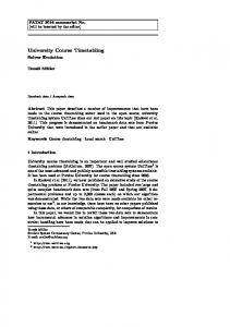
4.2. Comparative Results with time limits 4.2.1. Comparative results for the real test problem Based upon the results acquired from the implementation of the linear integer model using the CPLEX over the data of the real test problem, we obtained the values of as 736, 3.54, 51 and 27. Also, we obtained vales of using a long run of MS and SS 413, 257.63, 95 and 49. Figure 5 shows the objective algorithm as function’s improvement of different solution methods over the time. At the beginning, CPLEX has the worst objective cost but it has been improved quickly. Although CPLEX cannot find a better solution than SS during 3600 seconds of CPU time, but it surpasses the MA after 600 seconds of CPU time. Furthermore, we conclude that SS performs better than MA in all time limits and also, the best solution has been obtained by the SS.

265

Objective Function


CPLEX MA SS

0.45 0.4 0.35 0.3 0.25 0.2 0.15 0.1 0.05 0 0

500

1000

1500

2000

2500

3000

3500 time (s)

Figure 5: Comparative results for the real test problem

4.2.2. Comparative results for the theoretical test problems Similar to the previous section, we first calculate the values of which are reported in Table 8. Table 8: The values of SD 100

0.75

0.5

Test problem# 1 1 2 3 4 5 6 7 8 9 10 1 2 3 4 5 6 7 8 9 10

736 732 734 736 718 731 716 728 734 735 717 723 729 717 717 705 720 725 729 717 729

395 397 395 399 397 397 397 405 395 395 411 401 401 403 395 395 395 395 395 411 395

1.067 1.067 1.067 1.067 1.067 1.067 1.067 3.067 1.067 1.067 3.428 1.067 1.067 1.142 1.067 1.067 1.067 1.067 1.067 3.428 1.067

and

for all

1,2,3 and 4

and

267.62 250.27 246.86 251.08 265.08 257.97 246.55 240.37 251.11 258.86 234.963 252.64 229.49 236.42 246.18 246.48 232.49 241.29 242.11 213.523 235.10

51 51 51 51 56 51 55 56 52 51 52 52 56 59 55 54 52 52 51 52 52

97 97 97 96 94 97 91 91 97 96 81 97 97 91 97 94 94 96 97 82 94

27 27 27 27 28 27 27 28 27 27 27 27 29 28 27 27 27 27 27 27 27

49 49 49 49 49 49 49 49 49 49 49 49 49 49 49 49 49 49 49 49 49

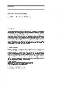
Figures 6, 7 and 8 indicate over different time limits, how the objective function is being improved

266


Objective Function

by different solutions approaches. In Figure 6, the improvement trends for all three solutions algorithms are almost similar to Figure 5 but this time, the CPLEX surpasses the MA after 900 seconds. Also, the best solution has been found by the SS.

CPLEX

0.45 0.4 0.35 0.3 0.25 0.2 0.15

MA SS

0.1 0.05 0 0

500

1000

1500

2000

2500

3000

3500 time (s)

Figure 6: Comparative results for the test problem with SD=1

Objective Function

Since for SD=0.75 and 0.5, we have 10 test problems, the average of objective functions over 10 test instances has been reported in Figures 7 and 8, respectively. 0.45 0.4 0.35 0.3 0.25

0.2 CPLEX 0.15 MA 0.1 SS 0.05 0 0

500

1000

1500

2000

2500

3000

3500

time (s)

Figure 7: Comparative results for the test problems with SD=0.75

267

Objective Function

Memetic and scatter search metaheuristic algorithms for a … 0.35 0.3 0.25 0.2 0.15

CPLEX MA

0.1

SS

0.05 0 0

500

1000

1500

2000

2500

3000

3500

time (s)

Figure 8: Comparative results for the test problems with SD=0.5

Figure 7 indicates that the SS algorithm has the best performance among three proposed solution approaches but Figure 8 reveals that CPLEX has surpassed the MA and SS algorithms after end of maximum time limit. By comparing the trend of improvements in three previous figures, we conclude that for harder test instance (higher value of SD) and for shorter time limits, the MA and SS have better performance that CPLEX but when the SD is decreased or the given time limit is increased, CPLEX is able to find better solutions that MA and SS. Tables 9 and 10 report the attained values for different objective functions over test problems with SD=0.75 by the MA and SS, respectively. These results have been obtained by the time limits TL=300 seconds. Table 9: Objective functions values obtained by MA over test problems with SD=0.75 in 300 seconds f1 f2 f3 f4 f 634 12.30 54 40 0.13 650 16.15 60 29 0.15 686 46.71 65 29 0.16 640 43.62 56 35 0.13 604 40.46 55 30 0.16 682 51.68 61 36 0.17 622 45.53 57 34 0.11 612 12.37 56 35 0.13 587 21.66 58 29 0.14 661 53.21 55 33 0.20

268

Movahedfar, Ranjbar, Salari, and Rostami Table 10 : objective functions values obtained by SS over test problems with SD=0.75 in 300 seconds f2 f3 f4 f f1 635 11.25 54 40 0.13 658 39.64 61 28 0.14 684 32.22 65 30 0.16 664 45.20 57 39 0.15 621 28.99 56 27 0.10 686 75.86 56 40 0.19 638 30.22 56 34 0.07 615 8.40 57 32 0.11 591 10.30 63 27 0.11 636 50.99 54 30 0.17

4.2.3. Statistical comparisons In order to have a more meticulous comparison of the three developed solution approaches, we have developed a statistical comparisons based on randomized complete block designs (Montgomery 2012). In particular, for each value of SD, we perform a statistical test in which different solution approaches and time limits are considered as treatments and blocks, respectively. For the real test problem and the randomly generated instances with SD=1, we have only one replication (one test problem) while for random instances with SD=0.5 and 0.75, totally 20 replications corresponding to 20 test problems, are available. We denote as "rp" the number of replications. In all of the four MA SS aforementioned statistical tests, the null hypothesis is : CPLEX and the alternate CPLEX MA SS hypothesis is : in which , and indicate the average performance of CPLEX, MA and SS over the corresponding instances, respectively. Table 11 reports the analysis of variance (ANOVA) in which , , and denote, respectively, the total corrected sum of squares, sum of squares of the differences between the treatments averages and the grand average, sum of squares of the difference between the blocks average and the grand average and . sum of squares errors, obtained by subtraction. In other words, we have , and denote the mean squares of treatments, blocks and errors, respectively. Also, The test statistic corresponding to and is which has F-distribution. The ANOVA corresponding to the real test problem is shown in Table 12 for which the Table 11: ANOVA table Source of deviation

Sum of squares

Degree of freedom

Treatments (algorithms)

3-1=2

Blocks (time limits)

9-1=8

Error

27rp-11

Total

27rp-1

Mean squares 2 8 27

11

P-value is around 0.03. Also, if we use the paired t-tests for pair comparisons of the three solution : , : and : the approaches, for statistical tests corresponding P-values are 0.048, 0.026 and 0.008, respectively. These results indicate that for the

269


real test problem, the difference between algorithms performance is not significant especially for two algorithms MA and SS. Table 12: ANOVA corresponding to the real test problem Source of deviation

Sum of squares

Degree of freedom

Mean squares


0.028

3-1=2

0.014


0.056

9-1=8

0.007

Error

0.051

27-11=16

0.003

Total

0.135

27-1=26

4.39

Similar to the real test problem, we develop Table 12 for the ANOVA of the theoretical test with SD=1 in which the P-value is again around 0.03. Also, If we use the paired t-tests for pair , : comparisons of the three solution approaches, for statistical tests : and : the corresponding P-values are 0.047, 0.023 and 0.04, respectively. Table 13: ANOVA corresponding to the test problem with SD=1 Source of deviation

Sum of squares

Degree of freedom

Mean squares


0.024

3-1=2

0.012


0.033

9-1=8

0.004

Error

0.043

27-11=16

0.0026

Total

0.1

27-1=26

4.49

Tables 14 and 15 represent the ANOVA for test instances with SD=0.75 and 0.5, respectively. Since number of replications is 10, the degrees of freedoms are changed. Table 14 indicates that the performance of the three developed algorithms are significantly different such that the P-value of this statistical test is approximately zero. Thus, we establish three paired t-tests to compare more exactly the solution approaches. For test problems with SD=0.75, the P-values of statistical tests : , : and : are all approximately zero which indicates they have significantly different performance. Table 14: ANOVA corresponding to the test problem with SD=0.75 Source of deviation

Sum of squares

Degree of freedom

Mean squares


0.217

3-1=2

0.108


0.621

9-1=8

0.078

Error

0.93

259

0.0036

Total

1.768

269

30

Analysis of the results of Table 15 is exactly similar to our analysis over the results of Table 13 and we conclude exactly the same P-values and conclusions. Finally, we conclude that performance of the three solutions approaches (i.e. CPLEX, MA and SS) are not significantly different for easier test problems (test problems with higher value of SD) but they show different performance on harder instances in which SS has the best performance and the

270


CPLEX has the worst performance. Table 14: ANOVA corresponding to the test problem with SD=0.5 Source of deviation

Sum of Squares

Degree of Freedom

Mean Squares


0.045

3-1=2

0.0225

Blocks (Time limits)

0.287

9-1=8

0.036

Error

0.427

259

0.0016

Total

0.759

269

14.06

5. SUMMARY AND CONCLUSIONS In this paper, we considered a case study of the fortnightly university course timetabling problem. We developed an integer linear programming model in which four different objective functions are combined into a single objective using the -metric method. We solved the developed model using CPLEX 12.3. Moreover, we developed a MA and a SS to solve the problem. For harder test problems and in shorter time limits, the metaheuristic algorithms have better performance than the CPLEX while SS outperforms always the MA. We showed this conclusion by the statistical tests as well. By decreasing the stretchability degree or complexity of test problems and in larger time limits, the CPLEX is able to surpass the developed metaheuristic algorithms. Since exact methods are unable to solve such a hard problem, developing heuristic or other metaheuristic solution techniques can be interesting research topics. REFERENCES: [1]

Alkan A, Ozcan E (2003), Memetic algorithms for timetabling; Proc. of IEEE Congress on Evolutionary Computation; 1796–1802.

[2]

Bagchi T P (1999), Multi-objective scheduling by genetic algorithms; Kluwer Academic Publishers.

[3]

Bardadym V A (1996), Computer-aided school and university timetabling: The new wave. In E. Burke & P. Ross (Eds.), Practice and theory of automated timetabling; Lecture notes in computer science 1153; 22–45, Berlin: Springer.

[4]

Belton V, Stewart T J (2002), Multiple criteria decision analysis - An Integrated Approach; Kluwer Academic Publishers.

[5]

Boland N, Hughes B D, Merlot L T G, Stuckey P J (2008), New integer linear programming approaches for course timetabling; Computers & Operations Research 35(7); 2209-2233.

[6]

Burke E K, Eckersley A J, McCollum B, Petrovic S, Qu R (2010), Hybrid variable neighborhood approaches to university exam timetabling; European Journal of Operational Research 206(1); 46-53.

[7]

Brucker P, Drexl A, Mohring R, Neumann K, Pesch E (1999), Resource-constrained project scheduling: notation, classification, models and, methods; European Journal of Operational Research 112; 3-41.

[8]

Burke E K, McCollum B, Meisels A, Petrovic S, Qu R (2007), A graph-based hyper heuristic for timetabling problems; European Journal of Operational Research 176(1); 177–192.

[9]

Ceschia S, Di Gaspero L, Schaef A (2012), Design, engineering, and experimental analysis of a simulated annealing approach to the post-enrolment course timetabling problem; Computers & Operations Research 39(7); 1615-1624.


271

[10]

Daskalaki S, Birbas T (2005), Efficient solutions for a university timetabling problem through integer programming; European Journal of Operational Research 160(1); 106-120.

[11]

Daskalaki S, Birbas T, Housos E (2004), An integer programming formulation for a case study in university timetabling; European Journal of Operational Research 153(1); 117-135.

[12]

Ehrgott M, Gandibleux X (2000), A survey and annotated bibliography of multi-objective combinatorial optimization; OR Spectrum 22(4); 425-460.

[13]

Glover F (1977), Heuristics for integer programming using surrogate constraints; Decision Sciences 8; 156-166.

[14]

Holland J H (1975), Adaptation in natural and artificial systems; Univ. Mich. Press.

[15]

Ishibuchi H, Yoshida T, Murata T (2002), Selection of initial solutions for local search in multiobjective genetic local search; Proceedings of the 2002 Congress on Evolutionary Computation (CEC 2002), IEEE Press; 950-955.

[16]

Jones D F, Mirrazavi S K, Tamiz M (2001), Multi-objective meta-heuristics: an overview of the current state-of-the-art; European Journal of Operational Research 137(1); 1-9.

[17]

Krasnogor N (2002), Studies on the theory and design space of memetic algorithms. Ph.D. Thesis; University of the West of England, Bristol, United Kingdom.

[18]

Laguna M, Marti´ R (2003), Scatter search—methodology and implementations in C; Kluwer Academic Publishers, Boston.

[19]

Lewis R (2008), A survey of metaheuristic-based techniques for university timetabling problems. OR Spectrum 30 (1); 167–190.

[20]

Lü Z, Hao J K (2010), Adaptive Tabu search for course timetabling; European Journal of Operational Research 200(1); 235-244.

[21]

Mirhassani S A (2006), A computational approach to enhancing course timetabling with integer programming; Applied Mathematics and Computation 175(1); 814-822.

[22]

Mitchell M (1998), An introduction to genetic algorithms (Complex Adaptive Systems); A Bradford Book.

[23]

Montgomery D C (2012), Design and analysis of experiments; Springer.

[24]

Neri F, Cotta C, Moscato P (2011), Handbook of memetic algorithms; Springer.

[25]

Paechter B, Rankin R C, Cumming A, Fogarty T C (1998), Timetabling the classes of an entire university with an evolutionary algorithm; Proc. of Parallel Problem Solving from Nature (PPSN V); 865– 874.

[26]

Pinedo M (2008), Scheduling, theory, algorithms, and systems, 3nd Edition; Prentice-Hall.

[27]

Rosenthal R E (1985), Principles of multi-objective optimization; Decision Sciences 16; 133-152.

[28]

Shiau D F (2011), A hybrid particle swarm optimization for a university course scheduling problem with flexible preferences; Expert Systems with Applications 38(1); 235-248.

[29]

Tan K C, Lee T H, Khor E F (2002), Evolutionary algorithms for multi-objective optimization: performance assessments and comparisons; Artificial Intelligence Review 17; 253-290.

[30]

Triantaphyllou E (2000), Multi-criteria decision making methods: A comparative Study; Springer.

[31]

T’kindt V, Billaut J C (2002), Multicriteria scheduling: Theory, Models and Algorithms; Springer.

[32] Wang Y Z (2003), Using genetic algorithm methods to solve course scheduling problems; Expert Systems with Applications 25(1); 39–50.