New Modeling Approach and Validation of a Thermoelectric Generator Nabil Karami
Nazih Moubayed
Department of Mechanical Engineering Faculty of Engineering 1 Lebanese University, Tripoli, Lebanon Email:
[email protected]
Department of Electricity and Electronics Faculty of Engineering 1 Lebanese University, Tripoli, Lebanon Email:
[email protected]
Abstract—In this paper, a mathematical modeling of a Thermoelectric Module (TEM) is presented. The modeling is based on several studies presented in literature with some correction of mistaken equations. The presented model is developed using different approach taking into consideration the modeling of the Maximum Power Point (MPP) and the maximum efficiency of a TEM. The proposed approach is validated and simulated using a Simulink model.
I. Introduction Thermo-Electric Module (TEM) is a two-way solidstate energy converter. It converts heat energy onto electrical energy when used as Thermo-Electrical Generator (TEG) and converts electrical energy into heat when used as Thermo-Electrical cooler/heater (TEC). TEM are made of two dissimilar semi-conductors (n and p-type) pellets that are electrically joined in series, to increase the operating voltage, and thermally in parallel, to decrease the thermal resistance. Pellets are sandwiches between thermal ceramic plates. The only difference between the structure of TEC and TEG is the distance among pellets where they are more condensed in TEG in order to increase their efficiency [1]. The solid-state structure with no mechanical moving parts offers the benefits of compactness, stability, noiseless and reliability. Thermo-electrical effect was first observed by Seebeck in 1821, where electrical current can be generated from two dissimilar joined metal. In 1834, Peltier discovered that the passage of current through a junction of two different metal produces a heating and a cooling effects. The Seebeck and the Peltier effects was co-related by Thomson effects by merging the heating/cooling and the electrical current effects at different temperature gradient. TEM are mostly used as cooler/heater (TEC) due to the fact that their efficiency in generating power (TEG) is about 5%, unless used to recover waste heat dissipated from industrial machines or ... TEC are mostly used for small cooler (refrigerator) for medical vaccine, organic tissues and blood preservation. Also, used for thermal control and management of CPU, laser diode and automotive seat cooling/heating systems.
Fig. 1. TEM pellets
II. Thermo-electrical Phenomenon Five energy phenomena take place in the TEM pellets: (i) Joule heating, (ii) Thermal conduction, (iii) Peltier heating/cooling, (iv) Seebeck effect, and (v) Thompson effect. The last effect is small enough to be neglected in the next derivations [2]. A. Seebeck effect Seebeck effect is the generation of a difference of potential between two dissimilar material when imposed to a temperature gradient. The TEM Seebeck voltage, also called EMF and open-circuit voltage, is the multiplication of the Seebeck coefficient, α(V /K), with the temperature gradient applied on a pn pellet, and is expressed by: VOC = α∆T
where α = αp − αn and ∆T = Thot − Tcold For a TEM composed of N p-n pellets, the EMF of the TEM becomes: VT EM,OC = αtotal ∆T where αtotal = N α
978-1-4799-2399-1/14/$31.00 ©2014 IEEE
(1)
586
(2)
B. Peltier heating/cooling effect
A. TEG thermal modeling
This phenomenon results in a heat absorption / dissipation due to the flow of current through a junction of two dissimilar material. TEM Peltier effect is described as:
Along the length, L, of a pellet pair, the variation of heat flow is given by the conduction at a distance dx from the initial position x, where its differential equation can be derived as [4], [5]:
Qa/d = αtotal Thot/cold I
(3)
where, Thot/cold (K) is the hot and cold temperatures, and I(A) is the current passing through the material. C. Joule heating effect Joule heating is the phenomenon that appears when current flows through a resistive (semiconductor) element. The heat dissipated from this effect is described as: Qjoule = I 2 RT EM,E (4) where RE is the electrical resistance of the semiconductor.
dQp,n (x) = Qp,n (x + dx) − Qp,n (x) = IT2 EM dREp,n (x)
where Qp,n is the conduction heat flow and IT2 EM dREp,n (x) represents the joule heating generated by the flow of current, IT EM , in the partial resistance of length x of dx the p- and n-type, given by dREp,n (x) = ρp,n A p,n . p,n According to Equation 7 and Fourier heat given in Equation 5 and by using the temperature boundary condition Tp,n (0) = Thot and Tp,n (L) = Tcold , the heat conduction rate at the hot and the cold junctions of the n-type and p-type pellets are described as [6]:
D. Thermal conduction effect Also known as Fourier process, this phenomenon describes the thermal conductivity or resistivity through a material. The heat transfer of thermal conduction in a TEM is presented as:
Qp,n (x) = −
Ap,n dTp,n (x)
ρT ,p,n dx Ap An ∆T ' −( + )∆T = − ρT ,p Lp ρT ,n Ln RT
(5)
where, • Ap (m2 ) and An (m2 ) are the cross sectional area of pand n-type pellets • Lp (m) and Ln (m) are the length of p- and n-type pellets • ρT ,p (mK/W ) and ρT ,n (mK/W ) are the thermal resistivity of the p- and n-type respectively.
where, • RE,p and RE,n are the electrical resistance of the p- and n-type pellets • ρE,p (Ωm) and ρE,n (Ωm) are the electrical resistivity of the p- and n-type respectively.
2 Thot − Tcold IT EM RE,p − RT ,p 2 2 Thot − Tcold IT EM RE,p + Qp (L) = RT ,p 2
Qp (0) =
(8)
IT2 EM RE,n
Thot − Tcold − RT ,n 2 Thot − Tcold IT2 EM RE,n Qn (L) = + RT ,n 2 Qn (0) =
Introducing the Peltier terms αIT EM Thot and αIT EM Tcold at the two boundary points, the rate of heat transfer from the heat source to the single-couple TEG and from the device to the heat sink can be obtained as: (
Qhot = Qp (0) + Qn (0) + αIT EM Thot Qcold = Qp (L) + Qn (L) + αIT EM Tcold
Equation 9 is expended using Equation 8 as: Thot − Tcold IT2 EM RE Q = − + αIT EM Thot hot RT 2 2 Thot − Tcold IT EM RE + + αIT EM Tcold Qcold = RT 2
III. TEG Modeling The electrical resistance, RE (Ω), and the thermal resistance, RT (K/W ), of a p- and n-type pellets are given by [3]: Lp L RE = RE,p + RE,n = ρE,p + ρE,n n Ap An (6) ρ L ρ L T ,p p T ,n n RT = RT ,p kRT ,n = ρT ,p Lp An + ρT ,n Ln Ap
(7)
(9)
(10)
For N couple of pellets, Equation 10 becomes: Thot − Tcold IT2 EM RT EM,E − + αtotal IT EM Thot Q = hot RT EM,T 2 Thot − Tcold IT2 EM RT EM,E Q = + + αtotal IT EM Tcold cold RT EM,T 2 (11) where RT EM,T = RT /N is the total thermal resistance and RT EM,E = N RE is the total electrical resistance.
587
B. TEM electrical modeling The difference in the hot- and cold-side heat is equal to the electrical power generated by the TEG and is given by: PT EM = Qhot − Qcold = VT EM IT EM = VT EM,OC IT EM − IT2 EM RT EM,E
(12)
where VT EM,OC is the EMF defined in Equation 2. Therefore, the TEG output voltage is the difference between the EMF and the voltage loss due to the internal electrical resistance (see Figure 2), thus, a corrected equation of the ones published in [6], [7], [8], [9] is expressed as: VT EM = VT EM,OC − IT EM RT EM,E
(13)
Fig. 2. TEM equivalent electric model
The quadratic equation of power (Equation 12) is a parabolic function of the form Y = aX−bX 2 , that is physically available only for a > bX or αtotal ∆T > IT EM RT EM,E . It can be concluded from the previous equation that the power is zero on two points: 1- when IT EM = 0, case of open-circuit V 2- when IT EM = IT EM,SC = RT EM,OC , case of short-circuit T EM,E Locating the vertex of a parabola or locating the Maximum Power Point (MPP) is achieved by equating the derivative of the power versus current to zero [10], [11], VT EM,OC op,P = (14) IT EM = IT EM dPT EM 2RT EM,E =0
Fig. 3. Power curves vs. current and voltage
dIT EM
op,P
dPT EM dIT EM
where = VT EM,OC − 2IT EM RT EM,E and IT EM is the optimum current leading to the maximum power op,P calculated by replacing IT EM in Equation 12 as [12], [13], Pmax
op,P
IT EM =IT EM
=
VT2EM,OC 4RT EM,E
(15)
By replacing IT EM by (VT EM,OC − VT EM )/RT EM,E the same analysis of power in function of the TEG voltage leads to: 588
Fig. 4. Power and efficiency curves
PT EM =
VT EM,OC VT EM − VT2EM RT EM,E
It can be concluded from the previous previous equation that the power is zero in two points: 1- when VT EM = 0, case of short-circuit 2- when VT EM = VT EM,OC , case of open-circuit The maximum power is calculating by derivating the power with VT EM as:
op,P VT EM = VT EM dP
=
T EM dVT EM
V
=0
VT EM,OC 2
r
(16)
(17)
ηmax
The equations developed previously are validated using the Simulink block diagram presented in Figure 5. The model is simulated by varying the load resistance, Rload , from zero (case of short-circuit current) to 100Ω, and monitoring the behavior of the PEG output voltage, current, power and efficiency.
op,P
−2V
op,P
=
VT EM =VT EM
VT2EM,OC 4RT EM,E
TABLE I Numerical values used in Simulink model Variable name Value αp 4.3622e-5 V /K αn 1e-5 V /K ρE,p 3.94e-5 Ωm ρE,n 3.937e-5 Ωm Lp , Ln 1e-4 m Ap , A n 1e-7 m2 Thot 80 ◦ C Tcold 10 ◦ C RT EM,T 1500 K/W Rload 0 to 10K Ω N 127
(18)
Thus, from Equation 14 and 17, the maximum power is accomplished by placing a load resistor equal to the internal electrical resistance. C. TEG efficiency modeling The efficiency of the TEG is given by the ratio of the delivered electrical power over the heat power [14]: η=
VT EM,OC IT EM − IT2 EM RT EM,E
PT EM = Qhot
IT2 EM RT EM,E RT EM,T 2 (19) The curve representing the variation of efficiency versus the current is given in Figure 4. The efficiency is zero when the numerator of Equation 19 is zero, therefore, the efficiency is zero: 1- when IT EM = 0, case of no load 2- when IT EM = VT EM,OC /RT EM,E , case of short-circuit ∆T
(21)
IV. TEG Model Validation and Simulation Results
dPT EM T EM = T EM,OC and VT EM is the optimum where dV RT EM,E T EM output voltage leading to the maximum power expressed as:
Pmax
op,E
IT EM =IT EM
z 1 + (Thot + Tcold ) − 1 2 ∆T = r Thot z T 1 + (Thot + Tcold ) + cold 2 Thot
+ αtotal Thot IT EM −
The location of the maximum efficiency is found by dη = 0, therefore, the efficiency is maximized equating dI T EM at:
Description Seebeck coefficient of p-type Seebeck coefficient of n-type Electrical resistivity of the p-type Electrical resistivity of the n-type Length of p and n pellets Area of p and n pellets Hot temperature Cold temperature Thermal resistance Load resistance Number of np pellets
Simulation results, shown in Figures 7 and 6, show one MPP and one maximum efficiency point at different load resistance. Using the numerical parameters presented in Table I, a maximum power of 2.23 mW is reached at 15 mA when the load resistor is equal to 10 Ω i.e. equal to the internal resistance. The maximum efficiency is 4.41% located at a current of 14 mA and a load of 10.5 Ω. The efficiency of the a TEG increases when the thermal resistance increases. V. Conclusion A new modeling approach of a thermoelectric module is presented and validated in this paper. The proposed equations pave the way toward an easy implementation of a maximum power point tracker on TEG devices. The low efficiency of such devices make them suitable only for power regeneration of from waste heat. References
op,E IT EM
dη dIT EM
= =0
2 RT EM,T αtotal
(20) r ∆T Z ( 1 + (Thot + Tcold ) − 1) (Thot + Tcold ) 2
op,E
where IT EM is the optimum current leading to the α2
R
T em,T maximum efficiency and Z = total is the figure of RT EM,E merit. Replacing Equation 20 in Equation 19 solves the maximum efficiency as:
589
[1] DM Rowe and Gao Min. Evaluation of thermoelectric modules for power generation. Journal of Power Sources, 73(2):193–198, 1998. [2] Michael Freunek, Monika Müller, Tolgay Ungan, William Walker, and Leonhard M Reindl. New physical model for thermoelectric generators. Journal of electronic materials, 38(7):1214–1220, 2009. [3] D Champier, C Favarel, JP Bédécarrats, T Kousksou, and JF Rozis. Prototype combined heater/thermoelectric power generator for remote applications. Journal of Electronic Materials, pages 1–12, 2013. [4] Haruhiko Okumura and Satarou Yamaguchi. One dimensional simulation for peltier current leads. IEEE Transactions on Applied Superconductivity, 7(2):715–718, 1997.
Fig. 5. Simulink block diagram of the TEG model
Fig. 6. Voltage, Current, Power and Efficiency vs. load resistance
590
exchange membrane fuel cell. Journal of Fuel Cell Science and Technology, 10(5):14, 2013. [12] Shiho Kim, Sungkyu Cho, Namjae Kim, Nyambayar Baatar, and Jangwoo Kwon. A digital coreless maximum power point tracking circuit for thermoelectric generators. Journal of electronic materials, 40(5):867–872, 2011. [13] Jungyong Park and Shiho Kim. Maximum power point tracking controller for thermoelectric generators with peak gain control of boost dc–dc converters. Journal of electronic materials, 41(6):1242– 1246, 2012. [14] Emil Sandoz-Rosado and Robert J Stevens. Experimental characterization of thermoelectric modules and comparison with theoretical models for power generation. Journal of electronic materials, 38(7):1239–1244, 2009.
Fig. 7. Voltage, Power and Efficiency vs. Current
[5] Min Chen, Lasse A Rosendahl, Thomas J Condra, and John K Pedersen. Numerical modeling of thermoelectric generators with varing material properties in a circuit simulator. IEEE Transactions on Energy Conversion, 24(1):112–124, 2009. [6] Aarti Kane, Vishal Verma, and Bhim Singh. Temperature dependent analysis of thermoelectric module using matlab/simulink. In IEEE International Conference on Power and Energy, pages 632– 637. IEEE, 2012. [7] Huan-Liang Tsai and Jium-Ming Lin. Model building and simulation of thermoelectric module using matlab/simulink. Journal of Electronic Materials, 39(9):2105–2111, 2010. [8] Simon Lineykin and Sam Ben-Yaakov. Spice compatible equivalent circuit of the energy conversion processes in thermoelectric modules. In 23rd IEEE Convention of Electrical and Electronics Engineers, pages 346–349. IEEE, 2004. [9] Simon Lineykin and Shmuel Ben-Yaakov. Modeling and analysis of thermoelectric modules. IEEE Transactions on Industry Applications, 43(2):505–512, 2007. [10] Nabil Karami, Rachid Outbib, and Nazih Moubayed. Fuel flow control of a pem fuel cell with mppt. In IEEE International Symposium on Intelligent Control (ISIC), 2012, pages 289–294. IEEE, 2012. [11] Nabil Karami, Rachid Outbib, and Nazih Moubayed. Maximum power point tracking with reactant flow optimization of proton
591
Powered by TCPDF (www.tcpdf.org)