Modeling Customer-Side Distributed Energy Resources Dispatch ...

LBNL- 185943

Modeling Customer-Side Distributed Energy Resources Dispatch Optimization for Electric Grid Transactions Girish Ghatikar, Salman Mashayekh, Michael Stadler, Rongxin Yin and Zhenhua Liu Lawrence Berkeley National Laboratory Berkeley, CA

July 2015 The work described in this report was coordinated by the Demand Response Research Center and funded by the California Energy Commission (Energy Commission), Public Interest Energy Research (PIER) Program, under Work for Others Contract No. 500-03026, and by the U.S. Department of Energy under Contract No. DE-AC02-05CH11231. The authors acknowledge all those who assisted in review of this document, and for their ongoing support, including the Energy Commission and PIER Program staff.

Disclaimer This document was prepared as an account of work sponsored by the United States Government. While this document is believed to contain correct information, neither the United States Government nor any agency thereof, nor The Regents of the University of California, nor any of their employees, makes any warranty, express or implied, or assumes any legal responsibility for the accuracy, completeness, or usefulness of any information, apparatus, product, or process disclosed, or represents that its use would not infringe privately owned rights. Reference herein to any specific commercial product, process, or service by its trade name, trademark, manufacturer, or otherwise, does not necessarily constitute or imply its endorsement, recommendation, or favoring by the United States Government or any agency thereof, or The Regents of the University of California. The views and opinions of authors expressed herein do not necessarily state or reflect those of the United States Government or any agency thereof or The Regents of the University of California.

Modeling Customer-Side Distributed Energy Resources Dispatch Optimization for Electric Grid Transactions Rish Ghatikar, Salman Mashayekh, Michael Stadler, Rongxin Yin, and Zhenhua Liu Lawrence Berkeley National Laboratory

Abstract Clean energy generation and power systems in the United States are evolving to provide reliable energy to consumers. California’s energy generation goals require 33 percent of annual retail sales from renewable sources by 2020, and Rule 21 requires identification of customer-side distributed energy resources (DER) controls, communication technologies, and standards. While generation exists at various levels within a Smart Grid, the customer-side DER plays a key role for demand response (DR) options. The challenges include leveraging the existing DER technology infrastructure, and enabling optimized cost, energy, and carbon choices for customers to deploy grid transactions at scale. The report describes the ongoing study on cost-effective communication technologies for DER integration and interoperability using tools and open standards, as well as optimization models for resource planning based on day-ahead price notifications. It identifies architectures and customer engagement strategies in dynamic pricing DR transactions to generate a feedback model for load flexibility, load profiles, and participation schedules. The results show that the model fits within the transactive energy concepts of the GridWise Architecture Council for communication tools that coordinate entities to maximize social welfare with minimal engagement, and grid system operators to utilize customer-side DER for grid transactions.

1

Table of Contents 1.

Introduction and Background .............................................................................................................. 4

2.

Test Site, Resources, and Technology Integration............................................................................... 7

3.

4.

5.

2.1.

Demand Response Quick Assessment Tool .................................................................................. 7

2.2.

Distributed Energy Resource Customer Adoption Model ............................................................ 7

2.3.

Open Automated Demand Response Standards .......................................................................... 8

2.4.

Distributed Resource and Demand Response Program Integration............................................. 9

Case Studies and Simulation Results ................................................................................................. 10 3.1.

Fort Hunter Liggett Site ............................................................................................................... 11

3.2.

Case Study Setup and Assumptions ............................................................................................ 11

3.3.

Load Shed Potential of DR Resources in FHL .............................................................................. 12

3.4.

Optimization of DER and DR Integration for Real-Time Prices ................................................... 13

3.5.

Optimization of DER and DR Integration for Peak Day Pricing ................................................... 21

3.6.

Optimization of DER and DR integration for Transactive Energy ............................................... 27

Conclusions and Future Research ...................................................................................................... 28 4.1.

Benefits of this Study to California ............................................................................................. 29

4.2.

Future Research and Development ............................................................................................ 29

References .......................................................................................................................................... 30

2

ACKNOWLEDGEMENTS The work described in this report was coordinated by the Demand Response Research Center and funded by the California Energy Commission (Energy Commission), Public Interest Energy Research (PIER) Program, under Work for Others Contract No. 500-03-026, and by the U.S. Department of Energy under Contract No. DE-AC02-05CH11231. The authors acknowledge all those who assisted in review of this document, and for their ongoing support, including the Energy Commission and PIER Program staff.

DISCLAIMER This report was prepared as the result of work sponsored by the California Energy Commission. It does not necessarily represent the views of the Energy Commission, its employees or the State of California. The Energy Commission, the State of California, its employees, contractors and subcontractors make no warrant, express or implied, and assume no legal liability for the information in this report; nor does any party represent that the uses of this information will not infringe upon privately owned rights. This report has not been approved or disapproved by the California Energy Commission nor has the California Energy Commission passed upon the accuracy or adequacy of the information in this report.

3

1 Introduction and Background Clean energy generation and power systems in the United States (U.S.) are evolving to provide reliable energy to consumers. Some states have more aggressive clean and distributed generation (DG) goals. For example, California’s energy generation goals require 33 percent of annual retail sales from renewable sources by 2020, 12 gigawatts (GW) of DG by 2020, and one million solar rooftops by 2018 (CEC, 2015a). California Public Utilities Commission (CPUC) Rule 21 interconnection guidelines require identification of customer-side distributed energy resources (DER) and appropriate communication technologies and standards for grid connectivity (CPUC, 2015a). California will need over 4 GW of ancillary services (fast dispatch capabilities) and cost-effective energy storage to meet 2020 clean energy generation goals (Masiello et al., 2010). California was the first state in the U.S. to have an energy storage mandate of 1.3 GW of energy storage by 2020 (CPUC, 2015b). These issues are not going to be unique to California, as many U.S. states also have clean energy generation goals (e.g., New York, Hawaii), and they will be facing similar challenges over the next few years and demand response (DR) will continue to be an important tool to integrate variable generation. While electricity generation exists at various levels, customer-side DER plays a key role in enabling California to move toward its clean energy generation goals. There are four key challenges to using DER under such an environment: 1. Understanding the existing market mechanisms for DR and automation and their readiness for future electricity grid changes. 2. Understanding and leveraging the DER technology infrastructure to provide DR for current and future electricity markets. 3. Enabling a dynamic model-in-the-loop for optimized cost, energy, and carbon choices for customers to identify flexible loads and participate in DR transactions. 4. Providing dynamic feedback mechanisms between customers and utilities or electric grid operators for a reliable and persistent DR under different market mechanisms. The current DR programs offered by California utilities rely on predetermined DR values (e.g., 50 kilowatts) from the customer, typically under a dispatch and estimated once a year through audits and tests. The DR performance is calculated and settled after the DR event. This is a big problem if the customer does not deliver the committed DR, as utilities cannot rely on a reliable and persistent response. Here, reliability refers to customer’s DR performance that closely matches the predetermined DR values, and persistency refers to customer DR participation in all events with a reliable response. In an effort to have reliable responses, this project evaluates the role of dynamic model-in-the-loop simulations to identify customer’s DR strategies under different technology parameters, and to provide a feedback to DR service providers. We propose a modeling framework, test it at a real site, and propose schemes to improve reliability and persistence for the dispatch-based DR programs with a certain kilowatt (kW) reduction. These models can also be used to estimate DR potential for tariff-based dynamic pricing DR programs. 4

The specific objectives of this project were as follows: ● ● ●

●

Identify cost-effective communication technologies and data model formats for DR and DER integration and interoperability using tools and open standards. Optimize DER for planning, based on day-ahead prices to allow DR customers to participate in a California utility’s dispatch-based DR program. Demonstrate optimized sequences and technologies for customer-side DER, such as natural gasfired/biogas-fired combined heat and power (CHP), batteries/storage, photovoltaics (PV), heat storage, etc. Generate resource availability and schedule feedback to utilities, systems operators, and aggregators, and enable customer-side DER participation in DR markets.

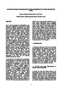
Figure 1 shows the existing DR and automation operation scenario compared to our proposed solution with customer-side DER. The key innovation is the customer day-ahead feedback of scheduled DR based on the results from the new model-in-the-loop simulations, which enables service providers to better plan their electricity purchase for the forecasted demand.

Figure 1: Existing DR operation scenario (left) and new operation scheme for DR/DER (right)

This report describes DR communication and automation technologies for DER integration and interoperability. We use the existing tools, open standards, and optimization models for resource planning to propose new models and feedback mechanisms based on a utility’s DR dispatches. This proposal empowers DR service providers with information on a customer’s load flexibility before the event is dispatched. The study demonstrated technologies that enable optimized cost and energy choices for customer-side DER for select automated DR (AutoDR) programs that are deployed by California utilities. We chose AutoDR because it does not involve human intervention, but rather is initiated at a building through the receipt of external communication signals (Piette et al., 2009a); and also because it has the potential to expand these models to “day-of” programs, to address faster response times through end-to-end-automation. Automation is needed for dynamic interactions between customers and the next-generation grid with a faster timescale of responses. We used the models at a real site and its DER technologies and day-ahead DR market signals for peak-day pricing (PDP) or critical-peak pricing (CPP) and real-time pricing (RTP). The transactive energy concepts are considered to optimize DER, and to identify load flexibility for energy markets.

5

Background In a continuing effort to meet the clean energy generation goals set forth by California, the renewable generation capacity, from both the grid (wholesale) and customers (self) was 21,000 megawatts (MW) (CEC, 2015b) at the end of 2014. This generation mix includes ~100,000 installations of solar PV (more than 1 gigawatt [GW] of solar PV) installed in 2011. In addition to local cost, energy, and carbon savings, one must consider the distributed generation resource’s ability to act as a DR resource for electric grid transactions. For DR and automation, over 250 MW is enrolled in California investor-owned and municipal utilities’ DR programs using a national and industry-supported open standard: OpenADR (Ghatikar et al., 2014). With increased adoption of DER such as CHP, storage, on-site generation, and others, there is a need to optimize DR planning based on multiple DR programs (e.g., day-ahead PDP/CPP and RTP) and standardized data models. The availability of DER to provide demand response to the existing utility DR programs depends on the timescales of DR and market requirements. Day-ahead dynamic prices can be considered to identify DR availability, and these are deployed by a majority of California’s AutoDR programs. For DR signals using open standards, we used OpenADR, which is used by California utilities for AutoDR programs. For optimization of dynamic model-in-the-loop, we used and integrated the distributed energy resource customer adoption model (DER-CAM). For optimization of customer’s DR strategies, we used the DR quick assessment tool (DRQAT). These technologies and tools were used in a simulated setup to assess the effectiveness and feasibility for customer-side DER participation in DR programs. Report Organization This report is organized into following sections: ● ● ●

Section 2 describes the site characteristics, loads, technologies, and tools used in the study, including their integration for dispatch-based DR programs. Section 3 describes the analysis results, including the setup and assumptions. Section 4 describes the conclusions and future work.

Research Methodology For the study, we identified the existing DR and DER technologies, tools, and program-specific system architecture for customers’ participation in dynamic DR transactions. A site (Fort Hunter Liggett army base) and the existing DR and DER optimization models were used as a case study. For test scenarios, we modeled California utilities’ AutoDR programs, which use open standards technologies for DR signals. The DER-CAM and DRQAT tools modeled local optimization of customer use of DER for DR programs. The final integrated tests and simulation runs were conducted to identify the models and generate feedback models for load flexibility, load profiles, and participation schedules, as well as to dynamically identify customer load flexibility, which both service providers and customers can use to determine DR reliability.

6

2 Test Site, Resources, and Technology Integration We used the following three key existing technologies and tools to develop models to enable DER integration with the grid and to enable its participation in existing DR programs.

2.1 Demand Response Quick Assessment Tool The Demand Response Quick Assessment Tool (DRQAT) is based on the modeling engine and capabilities of EnergyPlus (EnergyPlus, 2015). Users of DRQAT enter basic building information such as type, square footage, building envelope, orientation, utility schedule, etc. The assessment models use the prototypical simulation models to calculate energy and demand-reduction potential under certain DR strategies, such as pre-cooling, zone temperature setpoint adjustment, chilled water loop and air loop setpoint adjustment, and light dimming or on/off. DRQAT was used to develop models for simulating various DR strategies to estimate the kilowatt shed potential (Yin et al., 2010). We characterized DR control strategies at three levels (low, medium, and high) for each type of building. Each level of load shed potential was estimated using the DRQAT and was used as an input of load shed resource in DER-CAM (Figure 2).

Weather Data Building and HVAC DR Control Strategies

DER-CAM

Figure 2: Kilowatt shed potential from DRQAT to DER-CAM

2.2 Distributed Energy Resource Customer Adoption Model The Distributed Energy Resources Customer Adoption Model (DER-CAM), designed by Lawrence Berkeley National Laboratory (LBNL) and developed in the Generalized Algebraic Modeling System (GAMS), is a flexible decision-support tool for decentralized energy systems. Two major versions of this tool are available: (1) Investment & Planning DER-CAM, and (2) Operations DER-CAM. 1. Investment & Planning DER-CAM determines the optimal investment portfolio of DERs based on cost and performance characteristics, tariff information, and historic/simulated hourly load and PV generation data, from a given building, campus, or microgrid. 2. Operations DER-CAM provides detailed optimized operation schedules for existing DERs in a building or microgrid on a week-ahead basis, using forecasted loads and weather data. Operations DER-CAM is capable of running in 1-hour, 15-minute, 5-minute, or 1-minute time steps. In this project, we used the Operations version of DER-CAM. DER-CAM is mathematically modeled as a Mixed Integer Linear Program (Cardoso et al., 2014; Cardoso et al., 2013; Stadler et al., 2014; Stadler et al., 2013) and is based on the key premise that all thermal 7

and electrical loads are served, although specific actions leading to load shedding can also be considered. Figure 3 shows a high-level schematic of the energy flow in DER-CAM, in the form of a Sanky diagram.

Figure 3: Schematic of the energy flow model used in DER-CAM

To identify DR potential and send it to DER-CAM optimization, we used the existing tools: DRQAT to estimate kW shed potential and OpenADR for notification. Dynamic model-in-the-loop simulations were used to plan DR strategies, and notify the DR service provider on the estimated potential before the DR period was activated. We used the following key communications and technologies, since we had access to them. However, similar technologies can be used for other projects with similar concepts.

2.3 Open Automated Demand Response Standards Open Automated Demand Response (OpenADR), which is a U.S. standard, facilitates reliable and costeffective communication of electricity price and system grid reliability signals, allowing automated facility responses to dynamic prices. It provides non-proprietary, standardized interfaces to enable electricity service providers to communicate DR and DER signals to customers using a common language and existing communications (Piette et al., 2009b). The Virtual Top Node (VTN) and the Virtual End Node (VEN) are two major components in the interface of an OpenADR server, which allows hierarchy from the parent (the one that issues the primary DR signal) to the multiple parent/child relationships all the way to the end clients. Figure 4 shows the OpenADR communication diagram between the OpenADR server and the OpenADR client, which is integrated with DER-CAM.

8

OpenADR Server

PDP/RTP

OpenADR Client

DER-CAM

Figure 4: The OpenADR communication architecture

2.4 Distributed Resource and Demand Response Program Integration The project team set up an OpenADR server and client for an OpenADR test and DR integration research by providing OpenADR signal communications between the VTN and the VEN. The setup, which is based on the open source software, includes a fully featured server and interface that supports DR resources, market contexts, events, schedules, and reports. It is compatible with OpenADR 2.0a and 2.0b data profiles. In this study we created a client for DER-CAM to request the OpenADR signal from the OpenADR server. On the server side, we created an event for each DR program. Under each program, the OpenADR signal included signal type (e.g., price, level, and setpoint), time (start, end, and duration), current value, and signal ID. Figure 5 shows the schematic diagram of the closed-loop interactions between a DR service provider and a customer whose DER operation schedules are determined by DER-CAM. First, the DR service provider places the day-ahead OpenADR demand response signal on the OpenADR server. This signal contains the day-ahead RTP or PDP program information. Next, the OpenADR client (i.e., the customer) reads the signal from the server. The DR program information is then passed on to the Operations version of DER-CAM. As shown in Figure 5, other inputs to the customer’s Operations DER-CAM are the day-ahead weather, renewable generation, and load forecasts. After receiving all the required inputs, the DER-CAM optimization problem to minimize operation cost (or carbon dioxide emission) is solved. This determines the optimum operation schedules for the DERs and loads for the next day. The operation schedules are conveyed to an Energy Management and Controls System (EMCS), to change operations. A subset of the building’s operation schedules is sent to the OpenADR server, to be sent to the DR service provider.

9

Figure 5: Schematic diagram of the closed-loop interactions between a DR service provider and a DER-CAM-enabled customer

We selected two types of day-ahead DR programs in the case study: Peak Day Pricing (PDP) (PG&E, 2015a) and Real-Time Pricing (RTP) programs (SCE, 2015a, 2015b, and 2015c), which are offered by California utilities to their large commercial and industrial customers. While PDP is a dynamic pricing program, an RTP program provides flexible pricing schedules which are based on the season and the prior day’s temperature. A variant of the PDP program is a Critical Peak Pricing (CPP) program (PG&E, 2015a and 2015b), which is defined by a six-hour high-price DR period from 12 pm to 6 pm. The PDP program has a high price period from 2 pm to 6 pm with a typical 9 to 15 PDP event days per year, which are triggered during the hottest summer days. There are nine different pricing schedules for RTP: five for weekdays in summer, two for weekdays in winter, and two for weekends (summer or winter). The RTP demand response program structure and dispatch optimization within DER-CAM could also be used for continuous day-ahead hourly RTP signals. For the setup of those two DR programs, each pricing schedule was defined in VTN of the OpenADR server by creating each DR program event. For the RTP event setup, 24 hours of price signals were defined in an event, based on the outside air temperature of the prior day.

3 Case Studies and Simulation Results This section describes the case studies and discusses the results. After introducing the test site and the case assumptions, it describes how the load shed potential for the test site was obtained. The results for several RTP and PDP scenarios are presented and discussed. Finally, the links of this work to a transactive energy (TE) framework are discussed.

10

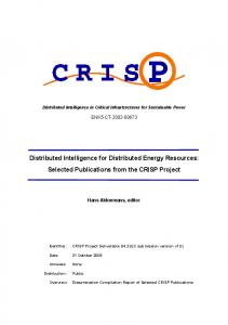
3.1 Fort Hunter Liggett Site Since LBNL has been working with Fort Hunter Liggett (FHL) for several years, and DER-CAM has been used there for optimum battery scheduling within a CPUC project, we used it as a simulation test case. Fort Hunter Liggett is the largest U.S. army reserve command post, covering about 162,000 acres in Monterey County, California (HDR, 2014). There are about 250 permanent civilian and military residents in this facility; however, the population can rise to 4,000 during troop training. It has a peak electrical load of 2.4 MW. Fort Hunter Liggett is home to 342 buildings with approximately 1.4 million square feet of space, including operational and training facilities, bed space, barracks, hotels, warehouses, offices, community support facilities, paved and graveled parking lots, recreational fields, parks, and open space areas (HDR, 2014). Figure 6 shows the electrical system configuration and technology portfolio at FHL. This includes 2 MW of solar photovoltaics connected to the system through four 500 kW inverters, 1 megawatt-hour (MWh) of lithium-ion (Li-ion) battery storage (2 units of 500 kilowatt-hour (kWh) / 625 kW), and several backup diesel generators adding up to 4 MW. Fort Hunter Liggett is served by Pacific Gas and Electric (PG&E) through 12 kilovolt (kV) lines. Low-voltage lines distributed throughout the facility are owned by FHL. Given the peak building demand of 2.4 MW, the battery storage can power all buildings for at least 25 minutes, which is normally enough for a backup generator to take over.

Utility Grid

Point of Common Coupling Breaker

4 MW Backup Diesel Several Units in 30-500 kW range

2 MW Solar Panel

1 MWh Battery

Building Loads

Figure 6: Electrical system configuration at FHL

3.2 Case Study Setup and Assumptions The load values shown in Figure 7 were used to forecast loads for the case studies. This figure shows the load in kW electrical for six different end uses (electrical only, cooling, refrigeration, space heating, water heating, and natural gas only) and two day types (non-peak weekdays and peak weekdays) in July. These curves were generated using some available historical data from FHL, along with some assumptions in terms of load shapes for the site.

11

1200 electricity-only.july.week 1000

electricity-only.july.peak cooling.july.week

Load (kW)

800

cooling.july.peak 600

refrigeration.july.week

400

refrigeration.july.peak space-heating.july.week

200

space-heating.july.peak 0 1 2 3 4 5 6 7 8 9 10 11 12 13 14 15 16 17 18 19 20 21 22 23 24

water-heating.july.week water-heating.july.peak

Time (Hours)

Figure 7: FHL loads for various end uses for normal weekdays and peak days in July (own estimations)

For PV forecasting, available measurements from PV panel generations at location (36°03'00.0"N, 120°33'00.0"W) in 2006 were used. This information is available in the “Solar Power Data for Integration Studies” database developed by the National Renewable Energy Laboratory (NREL) (NREL, 2014). As shown in Figure 8, this location is < 40 miles east of FHL.

Figure 8: PV generation data from a PV measurement site about 40 miles east of FHL

3.3 Load Shed Potential of DR Resources in FHL As mentioned above, the site has 312 buildings with approximately 2 million square feet of building area. Buildings include administration, schools, family housing, barracks, industrial/motorpool, dining, recreation, and other facilities. The lodging, office, and warehouse buildings constitute the majority of building areas on the site. DRQAT is developed for simulating individual building energy and demand performance. As we did not have detailed building data (e.g., building information, HVAC system, and related control capabilities), it was assumed that each category of building sector had the same load shed potential as the whole 12

building. The metric of DR shed percentage over the whole building (%WBP) was used to scale up an individual building case to the entire facility site. Three types of DR control strategies were evaluated (Table 1), using DRQAT to estimate the impact on load reduction during peak hours. For the “Global Temperature Adjustment” control strategy, three levels of temperature reset from the normal setpoint (e.g., 74F) were simulated to achieve the load shed from the whole building power by 5 percent, 10 percent, and 15 percent, respectively. For DR control of the lighting, it was assumed that lights in the daylight zone area could be shut down completely and lights in the interior zones could be dimmed by one-third and two-thirds as the mediumand high-level DR. By aggregating the high-level load shed potential of each control strategy, the highest load shed can reach 27 percent of the whole building power on the site. Table 1: Summary of load shed potentials for an individual building case DR Control Strategies Global Temp Adjustment

Lighting

Other Types of Load

Levels

DR Controls

%WBP (Whole Building Power)

Low

2F

5

Medium

4F

10

High

6F

15

Low

Dimming

2

Medium

Mixed

6

High

Shut Down

10

Medium

Shut Down

1

High

Shut Down

2

Other common DR strategies include cycling off rooftop units, shutting down water pumps or air compressors, and others. For a more specific case of load shed estimation, a detailed model would be required. This can be done by collecting more data from the site and using them to analyze each group of DR control strategies’ load shed potential.

3.4 Optimization of DER and DR Integration for Real-Time Prices In the RTP program, the DR service provider uploads the RTP hourly prices for the next day on the OpenADR server. For this study we used Southern California Edison (SCE) real-time price data, since PG&E does not offer an RTP program. The SCE-TOU-8 RTP values for 2–50 kV customers are listed in Table 2 (SCE, 2015a). An energy charge of $0.02463/kWh is also added to these hourly prices (SCE, 2015c). Also, there is a non-coincidental monthly demand charge of $14.88/kW for these customers. The prices are significantly different for different seasons/temperatures/days of the week, which provides great potential for optimization to 13

reduce energy cost. As an example, Figure 9 compares the hourly prices between hot weather and extremely hot weather tariffs. Table 2: SCE RTP prices for TOU-8 2–50 kV customers Summer Weekday

Winter Weekday

Summer/Winter Weekend

Extremely Hot Weather

Very Hot Weather

Hot Weather

Moderate Weather

Mild Weather

High Cost

Low Cost

High Cost

Low Cost

Temp. Range

≥ 95°F

91°F–94°F

85°F–90°F

81°F–84°F

≤ 80°F

> 90°F

≤ 90°F

≥ 78°F

< 78°F

1

0.05696

0.04632

0.04025

0.03789

0.03616

0.06199

0.04646

0.04860

0.04386

2

0.04983

0.03948

0.03405

0.03244

0.03168

0.05804

0.04165

0.04294

0.03801

3

0.04235

0.03284

0.02836

0.02674

0.02756

0.04998

0.03876

0.03830

0.03508

4

0.03766

0.03080

0.02602

0.02451

0.02489

0.05371

0.03839

0.03613

0.03151

5

0.03882

0.03307

0.02973

0.02697

0.02736

0.05726

0.04183

0.03592

0.03177

6

0.05242

0.04222

0.03643

0.03395

0.03401

0.07118

0.05154

0.03820

0.03455

7

0.05404

0.04505

0.04054

0.03692

0.03687

0.08257

0.05926

0.03623

0.03168

8

0.05815

0.05028

0.04610

0.04228

0.04194

0.08532

0.06321

0.03988

0.03394

9

0.06538

0.07125

0.05068

0.04856

0.04791

0.08188

0.06334

0.04686

0.04231

10

0.12247

0.10828

0.05670

0.05636

0.05479

0.09393

0.06497

0.05325

0.04739

11

0.28558

0.23340

0.07549

0.06176

0.05972

0.13529

0.06708

0.05791

0.05264

12

0.63062

0.37325

0.08603

0.06506

0.06229

0.17390

0.06718

0.06154

0.05439

13

1.03024

0.54524

0.11616

0.06760

0.06471

0.21225

0.06606

0.06219

0.05302

14

1.79778

0.88277

0.29203

0.07572

0.06766

0.29456

0.06615

0.06352

0.05062

15

2.60312

1.14253

0.47164

0.09752

0.07427

0.36877

0.06543

0.06733

0.05118

16

3.65591

1.47377

0.61301

0.12521

0.08070

0.42134

0.06533

0.06997

0.05190

17

3.65735

1.35294

0.62328

0.11394

0.07896

0.35774

0.06650

0.07616

0.05413

18

2.70390

1.02536

0.39304

0.08703

0.06855

0.23105

0.07089

0.08060

0.05748

19

1.69191

0.51948

0.21673

0.07809

0.06516

0.19774

0.07371

0.07786

0.05884

20

1.19066

0.34947

0.14721

0.06560

0.06154

0.20313

0.07392

0.07668

0.06230

21

1.31419

0.56959

0.14708

0.06829

0.06456

0.20683

0.07102

0.08442

0.06428

22

0.26068

0.21943

0.07573

0.06275

0.05993

0.10543

0.06568

0.06838

0.05964

23

0.07049

0.09144

0.05618

0.05561

0.05488

0.07412

0.05964

0.05855

0.05192

24

0.06234

0.05354

0.04831

0.04626

0.04448

0.06855

0.05078

0.05021

0.04357

RTP Energy Rates (USD / kWh)

Hour

4 3.5 3 2.5 2 1.5 1 0.5 0

Extremely Hot Hot

0

1

2

3

4

5

6

7

8

9

10 11 12 13 14 15 16 17 18 19 20 21 22 23 24 Time of Day (Hours)

Figure 9: Comparison of RTP rates for extremely hot weather and hot weather

14

In this project, we developed a new feature for Operations DER-CAM, where the customer sets the maximum daily energy cost (i.e., energy budget). This helps a customer limit its energy cost during highpriced days, granted its willingness to reduce some loads (the time and amount of load reduction is decided by DER-CAM). Another cost-limitation strategy is to set a maximum yearly cost. However, the inclusion of a maximum yearly cost in day-ahead optimization is challenging due to the mismatch in optimization time horizons. To set a maximum yearly cost, one needs to conduct pre-calculations (outside of DER-CAM) to obtain a maximum daily cost (for the optimization day) from the yearly cost goal using information with lots of uncertainties. In the following paragraphs, the new features are presented. The maximum daily energy cost constraint can be shown as follows: 24

∑ 𝑃𝑔𝑟𝑖𝑑 (𝑛) × 1ℎ𝑟 × 𝑅𝑅𝑇𝑃 (𝑛) ≤ 𝐶 𝑚𝑎𝑥 + 𝐶 𝑖𝑛𝑓𝑠𝑏

(Equation1)

𝑛=1

In Equation 1, 𝑃𝑔𝑟𝑖𝑑 (𝑛) is the customer’s grid power consumption in the n-th hour, 𝑅𝑅𝑇𝑃 (𝑛) is the RTP energy rate for the n-th hour, and 𝐶 𝑚𝑎𝑥 is the maximum allowed daily energy cost for the customer. The second term in the right-hand side of the equation, 𝐶 𝑖𝑛𝑓𝑠𝑏 , is used to keep the problem feasible, even if the set goal cannot be achieved after shedding all possible loads. For this purpose, the new term 𝐶 𝑖𝑛𝑓𝑠𝑏 × 𝐵 is added to the optimization objective function, as shown in Equation 2 and Equation 3 below, in which B is a very big number as the penalty term. 𝑛𝑒𝑤 𝑜𝑏𝑗𝑒𝑐𝑡𝑖𝑣𝑒 𝑓𝑢𝑛𝑐 = 𝑜𝑟𝑖𝑔𝑖𝑛𝑎𝑙 𝑜𝑏𝑗𝑒𝑐𝑡𝑖𝑣𝑒 𝑓𝑢𝑛𝑐 + 𝐶 𝑖𝑛𝑓𝑠𝑏 × 𝐵 𝐶 𝑖𝑛𝑓𝑠𝑏 ≥ 0 ,

𝐵 >> 0

(Equation 2) (Equation 3)

By including Equations 1–3, ● ●

if the maximum daily energy cost constraint can be met by using local generation, local storage, load shifting, and load curtailment, then 𝐶 𝑖𝑛𝑓𝑠𝑏 will be zero; otherwise, if the available resources are not enough to meet the goal, 𝐶 𝑖𝑛𝑓𝑠𝑏 will be non-zero, and its values will be the extra energy cost above the set goal.

To simulate an RTP event, the following steps are taken: ● ● ● ● ●

A date is chosen. Values from the NREL database for 2006 PV generation for the same day of the year are used as the PV generation forecast for the chosen date. Load values from a peak day in the month are used as the load forecast. A maximum daily energy charge is set. The DER-CAM optimization is run, and the results are analyzed. 15

For the following analysis, load and PV values were chosen for a summer day on July 22. The customer’s optimal dispatch was obtained for three storage capacities of 1,000, 2,000, and 5,000 kWh, and for three types of weather temperatures: hot, very hot, and extremely hot. In the first set of studies, whose results are summarized in Figure 10, no energy cost limits, i.e., 𝐶 𝑚𝑎𝑥 in Equation 1, were set. Consequently, no load reduction was carried out. For each tariff type (i.e., hot weather, very hot weather, and extremely hot weather) and each storage size (i.e., 1,000, 2,000, and 5,000 kWh), this figure shows daily electricity purchase, peak (2 pm–6 pm) electricity purchase, and daily energy cost (excluding demand charges). It can be seen that when a small battery (i.e., 1,000 or 2,000 kWh) is used, the customer’s electricity purchase during 2 pm–6 pm remains the same. More generally, the customer’s utility consumption and battery charging/discharging strategy remains almost the same during the entire day, as shown in Figure 11. This is due to the lack of available resources. In other words, the customer does not have flexibility to manipulate the resources, and hence, the optimal strategy remains the same regardless of the energy rates. 18000 16000 14000 12000 10000 8000 6000 4000 2000 0 Hot

Very Hot

Ex. Hot

Batt. Cap. 1000 kWh

Hot

Very Hot

Ex. Hot

Batt. Cap. 2000 kWh

Hot

Very Hot

Ex. Hot

Batt. Cap. 5000 kWh

Electricity Purchase (kWh)

13300

13400

13354

13000

13000

13002

12400

12400

12400

Electricity Purchase in 2-6 pm (kWh)

3137

3137

3100

2858

2858

2682

2140

2140

1391

RTP Energy Cost ($)

2950

6850

16164

2750

6340

14396

2280

5160

9190

Figure 10: Electricity purchase and RTP energy cost versus RTP tariff day type and battery size without energy cost limitation. Analysis carried out in DER-CAM.

16

Energy from Utility (kWh)

1000 800 600 400 Extremely Hot Hot

200 0 0

1

2

3

4

5

6

7

8

9

10 11 12 13 14 15 16 17 18 19 20 21 22 23 24 Time of Day (Hours)

Battery State of Charge (%)

(a) Utility energy consumption 1.2 1 Extremely Hot Hot

0.8 0.6 0.4 0.2 0 0

1

2

3

4

5

6

7

8

9

10 11 12 13 14 15 16 17 18 19 20 21 22 23 24 Time of Day (Hours)

(b) Battery state of charge Figure 11: Comparison of optimal dispatch for extremely hot weather tariff vs. hot weather tariff, for a 1,000 kWh battery without energy cost limitation. Analysis carried out in DER-CAM.

For a bigger battery, i.e., 5,000 kWh, Figure 10 shows that the customer is able to reduce the peak consumption from 2,140 kWh for hot weather and very hot weather tariffs to 1,391 kWh for an extremely hot weather tariff. The difference between the optimal utility consumption and the battery charging/discharging strategy for hot weather and extremely hot weather tariffs are depicted in Figure 12. It shows that the customer uses more energy from the battery and less energy from the utility when the energy rates are very high.

17

Energy from Utility (kWh)

700 600 500 400 300 200

Extremely Hot Hot

100 0 0

1

2

3

4

5

6

7

8

9

10 11 12 13 14 15 16 17 18 19 20 21 22 23 24 Time of Day (Hours)

Battery State of Charge (%)

(a) Utility energy consumption 1.2 1 Extremely Hot Hot

0.8 0.6 0.4 0.2 0 0

1

2

3

4

5

6

7

8

9

10 11 12 13 14 15 16 17 18 19 20 21 22 23 24 Time of Day (Hours)

(b) Battery state of charge Figure 12: Comparison of optimal dispatch for extremely hot weather tariff vs. hot weather tariff, for a 5,000 kWh battery without energy cost limitation. Analysis carried out in DER-CAM.

In the second set of studies, a maximum energy cost was set for the optimization day. The maximum energy cost was arbitrarily set to 1.5 times the daily energy cost with the hot weather tariff. The load reduction was also allowed in this set of studies, and the maximum load reduction potential was set to 27 percent for the electrical and cooling loads, based on the load shed potential studies reported in Section ‎3.3. Figure 13 shows a summary of the results. Note that the cases with a hot weather tariff are the same as those in Figure 10. Figure 13 shows that the daily electricity purchase and the 2 pm–6 pm electricity purchase decrease as the energy rates increase from hot weather to very hot weather to extremely hot weather tariffs. The load reduction increases as the energy rates increase. Table 3 shows the RTP energy costs, in U.S. dollars (USD) and percent with respect to the hot weather tariff price, for various cases. The maximum energy cost limitation is met for all storage sizes, when the very hot weather tariff rates are used. However, with extremely hot weather tariff rates with 1,000 and 2,000 kWh batteries, the energy cost goal cannot be satisfied, since the load reduction potential is not big enough. For a 5,000 kWh battery, however, this goal is met, and the daily energy cost is limited to 150 percent of the cost with the hot weather tariff.

18

14000 12000 10000 8000 6000 4000 2000 0

Very Hot

Hot

Ex. Hot

Batt. Cap. 1000 kWh Electricity Purchase (kWh)

13300

12100

Electricity Purchase in 2-6 pm (kWh)

Very Hot

Hot

Ex. Hot

Batt. Cap. 2000 kWh

9480

13000

12400

Hot

Very Hot

Ex. Hot

Batt. Cap. 5000 kWh

9200

12400

12352

10600

3137

1210

903

2858

959

154

2140

460

0

Load Reduction (kWh)

0

1260

3840

0

763

3840

0

0

1710

RTP Energy Cost (USD)

2950

4430

6670

2750

4130

4510

2280

3420

3420

Figure 13: Electricity purchase and RTP energy cost versus RTP tariff day type and battery size with energy cost limitation. Analysis carried out in DER-CAM. Table 3: RTP energy cost for cases with energy cost limitation. Analysis carried out in DER-CAM. Battery Size

1,000 kWh

2,000 kWh

5,000 kWh

Hot Weather

Very Hot Weather

Ex. Hot Weather

Hot Weather

Very Hot Weather

Ex. Hot Weather

Hot Weather

Very Hot Weather

Ex. Hot Weather

RTP Energy Cost (USD)

2,950

4,430

6,670

2,750

4,130

4,510

2,280

3,420

3,420

RTP Energy Cost (%)

100%

150%

226%

100%

150%

164%

100%

150%

150%

RTP Day Type

Figure 14(a)–(c) show the utility energy consumption, battery state of charge, and load reduction, respectively, for hot weather and extremely hot weather day type tariffs, when the battery capacity is 1,000 kWh and the energy cost is limited. In Figure 14(c), the dashed line shows the load reduction potential, i.e., 27 percent of the total load, for the site. This figure shows that the entire load reduction potential is being used during high-energy-cost periods. However, as shown in Table 3, the energy cost goal cannot be achieved, due to the small size of the battery.

19

Energy from Utility (kWh)

1000 900 800 700 600 500 400 300 200 100 0

Extremely Hot Hot

0

1

2

3

4

5

6

7

8

9

10

11

12

13

14

15

16

17

18

19

20

21

22

23

24

Time of Day (Hours)

Battery State of Charge (%)

(a) Utility energy consumption 1.2 1 Extremely Hot Hot

0.8 0.6 0.4 0.2 0 0

1

2

3

4

5

6

7

8

9

10 11 12 13 14 15 16 17 18 19 20 21 22 23 24 Time of Day (Hours)

(b) Battery state of charge

Load Reduction (kWh)

600 Load Reduction - Extremely Hot

500 400 300 200 100 0 0

1

2

3

4

5

6

7

8

9

10 11 12 13 14 15 16 17 18 19 20 21 22 23 24 Time of Day (Hours)

(c) Load reduction Figure 14: Comparison of optimal dispatch for extremely hot weather vs. hot weather tariffs, for a 1,000 kWh battery with energy cost limitation. Analysis carried out in DER-CAM.

Figures 15(a)–(c) compare the utility energy consumption, battery state of charge, and load reduction, respectively, between hot weather and extremely hot weather day type tariffs, when the battery capacity is 5,000 kWh and the energy cost is limited. Figure 15(c) shows that in this case, the entire load reduction potential during high-energy-cost periods is not being used. However, as shown in Table 3, the energy cost goal is achieved, since the battery is big enough to provide enough flexibility.

20

Energy from Utility (kWh)

1200 1000 800 600 400 200

Extremely Hot Hot

0 0

1

2

3

4

5

6

7

8

9

10 11 12 13 14 15 16 17 18 19 20 21 22 23 24 Time of Day (Hours)

Battery State of Charge (%)

(a) Utility energy consumption 1.2 1 Extremely Hot

0.8 0.6 0.4 0.2 0 0

1

2

3

4

5

6

7

8

9

10 11 12 13 14 15 16 17 18 19 20 21 22 23 24 Time of Day (Hours)

(b) Battery state of charge

Load Reduction (kWh)

600 Load Reduction - Extremely Hot Load Reduction - Hot Load Reduction Potential

500 400 300 200 100 0 0

1

2

3

4

5

6

7

8

9

10 11 12 13 14 15 16 17 18 19 20 21 22 23 24 Time of Day (Hours)

(c) Load reduction Figure 15: Comparison of optimal dispatch for extremely hot weather vs. hot weather tariffs, for a 5,000 kWh battery with energy cost limitation: (top), (middle), (bottom). Analysis carried out in DER-CAM.

3.5 Optimization of DER and DR Integration for Peak Day Pricing For a PDP program, it is assumed that the DR service provider sends the OpenADR signal, which includes the requested reduction in the customer’s electricity consumption (from the grid) during the next day’s peak hours, e.g., 2 pm–6 pm. The requested reduction cannot exceed the amount agreed upon in the PDP participation contract between the two parties. 21

For the PDP case studies, energy rates and demand charges shown in Table 4 are mainly based on SCE’s TOU-8 CPP program (SCE, 2015c). This table shows that the customers get a much lower on-peak demand charge ($11.82/kW/month cheaper) if they participate in the PDP program. However, the energy rates during the on-peak period of a PDP day are much higher than the non-PDP rate ($1.37453/kWh more expensive). Table 4: PDP prices for TOU-8 2–50 kV customers Cost Meter charge ($/month)

319.47

Summer on-peak monthly demand charge ($/kW/month)

24.15

Summer mid-peak monthly demand charge ($/kW/month)

6.66

Summer non-coincidental monthly demand charge ($/kW/month)

14.88

Winter non-coincidental monthly demand charge ($/kW/month)

14.88

Summer on-peak energy rate ($/kWh)

0.13908

Summer mid-peak energy rate ($/kWh)

0.08411

Summer off-peak energy rate ($/kWh)

0.06

Winter mid-peak energy rate ($/kWh)

0.08593

Winter off-peak energy rate ($/kWh)

0.06544

Extra energy charge during 2 pm–6 pm on PDP event days ($/kWh)

1.37453

Credits for on-peak demand charge for PDP program participation ($/kW/month)

-11.82

Energy Rates (USD / kWh)

Figure 16 compares the energy rates between peak and non-peak days and shows the enormous difference between the two rates during peak hours, e.g., 2 pm–6 pm. 1.6 1.4 1.2 1 0.8 0.6 0.4 0.2 0

Peak Rates Normal Rates

0

1

2

3

4

5

6

7

8

9

10 11 12 13 14 15 16 17 18 19 20 21 22 23 24 Time of Day (Hours)

Figure 16: Comparison of energy rates between peak and non-peak days

To determine the customer’s baseline for an event day, a “10 out of 10” model was used. In this model, the average of the customer’s grid electricity consumption from the past 10 non-PDP-event weekdays (hence, excluding weekends and PDP-event days) is used as the customer’s baseline for a PDP-event day.

22

In this project, a new feature was applied to Operations DER-CAM to accommodate the PDP loadreduction constraint. The following paragraphs present the new equations. The new constraint, for a reduction request, i.e., 𝛥𝑃 < 0, is shown in Equation 4. − 𝑃𝑔𝑟𝑖𝑑 (𝑛) − 𝑃𝑖𝑛𝑓𝑠𝑏 (𝑛) ≤ 𝑃𝑏𝑎𝑠𝑒𝑙𝑖𝑛𝑒 (𝑛) + 𝛥𝑃 , 15 ≤ 𝑛 ≤ 18, 𝛥𝑃 < 0

(Equation 4)

The PDP program is focused on load-reduction requests. A model for a load increase request was also developed in this work. A load increase request may be issued during over-generation periods. The equation for an increase request, i.e., 𝛥𝑃 > 0, is shown in Equation 5. + 𝑃𝑔𝑟𝑖𝑑 (𝑛) + 𝑃𝑖𝑛𝑓𝑠𝑏 (𝑛) ≥ 𝑃𝑏𝑎𝑠𝑒𝑙𝑖𝑛𝑒 (𝑛) + 𝛥𝑃 , 15 ≤ 𝑛 ≤ 18, 𝛥𝑃 > 0

(Equation 5)

In the above equations, 𝑃𝑔𝑟𝑖𝑑 (𝑛) is the customer’s grid power consumption in the n-th hour, 𝑃𝑏𝑎𝑠𝑒𝑙𝑖𝑛𝑒 (𝑛) is the baseline for the n-th hour, and 𝛥𝑃 is the requested power reduction/increase compared to the baseline. Also, 15 ≤ 𝑛 ≤ 18 shows the PDP event hours, i.e., 2 pm–6 pm. The second − + term in the left-hand side of each equation, 𝑃𝑖𝑛𝑓𝑠𝑏 (𝑛) or 𝑃𝑖𝑛𝑓𝑠𝑏 (𝑛), is used to keep the constraint feasible, even if it cannot be achieved after using all of the building resources for load reduction/increase. For this purpose, a new term has been added to the objective function, as shown in Equation 6, in which B is a very big number. 18 − + 𝑛𝑒𝑤 𝑜𝑏𝑗 𝑓𝑢𝑛𝑐 = 𝑜𝑟𝑖𝑔𝑖𝑛𝑎𝑙 𝑜𝑏𝑗 𝑓𝑢𝑛𝑐 + ∑ (𝑃𝑖𝑛𝑓𝑠𝑏 (𝑛) + 𝑃𝑖𝑛𝑓𝑠𝑏 (𝑛)) × 𝐵

(Equation 6)

𝑛=15

− + 𝑃𝑖𝑛𝑓𝑠𝑏 (𝑛) ≥ 0 , 𝑃𝑖𝑛𝑓𝑠𝑏 (𝑛) ≥ 0 ,

𝐵 >> 0

(Equation 7)

By including equations 4 through 7, ●

in a reduction PDP event, i.e., 𝛥𝑃 < 0, − ○ if the requested reduction can be met by using available resources, then 𝑃𝑖𝑛𝑓𝑠𝑏 (𝑛)’s will ○

be zero; otherwise, − if the available resources are not enough to deliver 𝛥𝑃, 𝑃𝑖𝑛𝑓𝑠𝑏 (𝑛)’s will be non-zero, and − 𝑃𝑖𝑛𝑓𝑠𝑏 (𝑛) > 0 will be the customer’s deviation from the desired reduction;

●

similarly, in an increase PDP event, i.e., 𝛥𝑃 > 0, + ○ if the requested increase can be met by using available resources, then 𝑃𝑖𝑛𝑓𝑠𝑏 (𝑛)’s will ○

be zero; otherwise, + if the requested increase cannot be delivered, 𝑃𝑖𝑛𝑓𝑠𝑏 (𝑛)’s will be non-zero, and + 𝑃𝑖𝑛𝑓𝑠𝑏 (𝑛) > 0 will be the customer’s deviation from the desired increase during the n-th

hour.

23

To simulate a PDP event, the following steps are taken: ● ● ● ●

●

A date is chosen. Values from the NREL database for 2006 PV generation for the same day of the year are used as the PV generation forecast for the chosen date. Load values from a peak day in the month are used as the load forecast. To set the baseline during PDP hours: ○ A DER-CAM optimization is run for each of the past 10 non-weekend days. ○ For each of the 10 days, PV forecasts are generated using the NREL database. ○ For each of the 10 days, load forecasts are generated using the load values from a weekday in the month. ○ The average of the electricity purchase for the 10 days is calculated, for each hour, as the baseline for that hour. ○ Note that the on-peak, mid-peak, off-peak, coincidental, and non-coincidental power demands from these 10 days are also passed to the optimization for the PDP day. The DER-CAM optimization is run, and the results are analyzed.

For the following studies, the summer day July 22 was chosen, and assumed to be a PDP event day. For the battery storage, two capacities—1,000 kWh and 2,000 kWh—were considered. For each case, DERCAM was run for the 10 weekdays leading to the PDP event day, and the results were used to obtain the baseline for the utility consumption reduction. Figure 17 shows the results for the case with 1,000 kWh of battery storage. Figure 17(a) shows the baseline for the utility consumption with the dashed line and the desired maximum load during the peak hours with the thick line. The desired maximum load is the baseline minus the desired reduction, which was about 53 kWh per hour in this case. It can be observed that the load reduction goal was met during 2 pm–5 pm, but not during 5 pm–6 pm. Figure 17(c) shows that the customer was unable to meet the desired utility energy consumption reduction during 5 pm–6 pm even though it used its entire loadreduction potential during this hour. Figure 17(a) also depicts what the utility purchase for this day would have been if non-peak rates were to be used, and shows that the utility purchase during peak hours would have been much higher with non-peak rates. This shows the effectiveness of the peak day prices on lowering the customer’s utility purchase.

24

Energy from Utility (kWh)

PDP Desired Max Load Energy from Utility - Peak Rates Energy from Utility - Normal Rates PDP Baseload

1200 1000 800 600 400 200 0 0

1

2

3

4

5

6

7

8

9

10 11 12 13 14 15 16 17 18 19 20 21 22 23 24 Time of Day (Hours)

Battery State of Charge (%)

(a) Utility energy consumption 1.2 Peak Rates Normal Rates

1 0.8 0.6 0.4 0.2 0 0

1

2

3

4

5

6

7

8

9

10 11 12 13 14 15 16 17 18 19 20 21 22 23 24 Time of Day (Hours)

(b) Battery state of charge

Load Reduction (kWh)

600 Load Reduction - Peak Rates Load Reduction - Normal Rates Load Reduction Potential

500 400 300 200 100 0 0

1

2

3

4

5

6

7

8

9

10 11 12 13 14 15 16 17 18 19 20 21 22 23 24 Time of Day (Hours)

(c) Load reduction Figure 17: Comparison of optimal dispatch for peak vs. normal weekday tariffs, with a 1,000 kWh battery. Analysis carried out in DER-CAM.

Figure 17(b) compares the battery state of charge in the peak rates case with the non-peak case rates, and shows that the battery state of charge goes from fully charged to fully discharged (minimum charge) during peak hours when the peak rates are used. Note that for a PDP event, the customer’s feedback to the DR server/utility could be whether the requested reduction could be met, and if it could not, what the average reduction would be. For this 25

case, the reduction in the first three peak hours is the requested 53 kWh, but in the fourth hour it has a 244 kWh increase with respect to the PDP baseline. Hence, in average, there is a 21 kWh increase, instead of the requested 53 kWh decrease. For the next case, the battery capacity was assumed to be 2,000 kWh. Figure 18 shows the results for this case. Figure 18(a) shows the baseline for the utility consumption with the dashed line and the desired maximum load during the peak hours with the thick green line. The desired utility purchase reduction was about 53 kWh per hour in this case. It can be observed that with the higher battery capacity of 2,000 kWh, the load reduction goal was met during the entire peak period, i.e., hours 14–18. Figure 18(a) also depicts what the utility purchase for this day would be if non-peak rates were to be used, and shows that the utility purchase during peak hours would have been much higher with nonpeak rates. Figure 18(b)–(c) show the battery state of charge and load reduction, respectively. For this case, the customer’s response was their ability to meet the requested reduction.

26

Energy from Utility (kWh)

1200

PDP Desired Max Load

1000 Energy from Utility - Peak Rates

800 600 400 200 0 0

1

2

3

4

5

6

7

8

9

10 11 12 13 14 15 16 17 18 19 20 21 22 23 24 Time of Day (Hours)

Battery State of Charge (%)

(a) Utility energy consumption 2.5 Peak Rates Normal Rates

2 1.5 1 0.5 0 0

1

2

3

4

5

6

7

8

9

10 11 12 13 14 15 16 17 18 19 20 21 22 23 24 Time of Day (Hours)

(b) Battery state of charge

Load Reduction (kWh)

600 Load Reduction - Peak Rates

500 400 300 200 100 0 0

1

2

3

4

5

6

7

8

9

10 11 12 13 14 15 16 17 18 19 20 21 22 23 24 Time of Day (Hours)

(c) Load reduction Figure 18: Comparison of optimum dispatch for peak vs. normal weekday tariffs, with a 2,000 kWh battery. Analysis carried out in DER-CAM.

3.6 Optimization of DER and DR integration for Transactive Energy The GridWise Architecture Council (GWAC) has developed a transactive energy (TE) framework for a common understanding to develop and advance TE among stakeholders (GWAC, 2015). According to the GWAC, TE refers to, “the use of a combination of economic and control techniques to improve grid reliability and efficiency.” The customer response strategies to RTP or PDP developed in this project 27

would provide customers with techniques to optimize DER scheduling and operations, and for participation in the TE markets for grid reliability. In this hypothetical framework, the customer may be provided with several sets of electricity prices for the next day and will return its forecasted next-day consumption based on each price set. Hence, from the customer’s optimization formulation point of view, the transactive energy framework can be seen as an iterative RTP or PDP framework demonstrated in this work.

4 Conclusions and Future Research In this study, we evaluated California’s clean energy generation goals and the role of distributed energy resources (DER) and demand response (DR) to enable better integration of variable renewable energy generation resources. In particular, this work addresses current market mechanisms and technology deployments that do not consider the opportunity to improve reliability and persistency of DR from customers with DER infrastructure. Demand response schedule and availability can provide reliable and persistent DR for different timescales of electricity markets. This understanding is critical for preparing California for electricity grid changes and enabling customer-side DER to participate in electricity market programs. The results show that we can optimize the DER dispatch mechanisms for electric grid transactions using the dynamic model-in-the-loop analysis. Such models can be optimized for cost, energy, and carbon choices determined by the customers to identify demand flexibility. While we used the existing and known technologies, standards, and tools, the models can be applied to any similar DER operation schemes. The models can be used with DR programs and future transactive energy (TE) concepts for continuous interactions between the electricity grid and customers. The project identified new DER optimization equations and terms to: ● ● ● ●

Calculate maximum daily energy cost constraints set by the user or a customer. This can also be extrapolated from a customer’s annual energy cost constraints. Indicate if the customer can meet the daily energy cost constraint by optimized management of the loads and DER. Accommodate load change constraints (increase or decrease) for utility prices. In the case of PDP, these features can be applied against load decrease scenarios. Indicate if the customer can meet the load change constraints by optimized management of the loads and DER.

The daily cost constraints and customer’s comfort or facility operation depends on the magnitude of service-level changes. Another key result from this study was integration of existing DR technologies and standards deployed by the California utilities for dynamic optimization of DER and their gridinterconnection for DR services. While OpenADR is used by all three investor-owned-utilities in California, new feedback models provide continuous optimization, status, and availability of customer’s resources for requested DR. The feedback models from customers to service providers include:

28

● ●

Customer’s daily utility or grid electricity purchase hourly profiles for next 24 hours. This information can be used to reliably measure the individual or aggregated demand. Average DR load changes against a baseline used by the utility.

4.1 Benefits of this Study to California This study helps California to: ● ● ● ●

Assist and identify existing California utility standardized interfaces for AutoDR and use that infrastructure to use DER to provide DR services. Enable a cost-effective AutoDR technology infrastructure and its interoperability with DER resources. Reduce the utility companies’ costs for development of infrastructures to implement, control, and manage DER for DR markets, thus reducing costs to California ratepayers. Enable customer choice to be maximized to the extent practical, influencing future choices through appropriate rate design, not through command-and-control.

4.2 Future Research and Development OpenADR reporting services provide standardized representation of customer energy usage information at different timescales, which can be used for baseline calculations and telemetry requirements of the wholesale DR markets. Addition of new feedback models from DER optimization will lead to OpenADR application in transactive energy and utilization of customer-side DER to participate in electricity markets. Future studies should consider the following: 







Improve the accuracy of results: These results should be confirmed under different customer sectors, DER operation scenarios, and customer flexibility parameters to leverage the value of participating in DR and transactive energy markets. Study the impacts of forecasting errors: Currently, the planning and optimization are based on forecasting, and there are errors associated but not handled explicitly. Incorporating with risk management will greatly complement the system. Application of models in field tests: The models developed in this study should be applied in actual field tests in buildings and improve the simulation results through calibration from actual performance. Another aspect that we did not consider in this study was the cost effectiveness for potential large-scale adoption. Cost-effective integrated system and power system communications: Understanding of power system and communication architecture, as well as storage costs, influences the economic value of DER interconnection in electricity markets.

29

5 References California Energy Commission (2015a), http://www.energy.ca.gov/portfolio/.

“Renewable

Portfolio

Standards,”

Available:

California Energy Commission (2015b), “Summary of Renewable Energy Installations Current and Planned in California,” Available: www.energy.ca.gov/renewables/tracking_progress/ documents/renewable.pdf. California Public Utilities Commission (2015a), http://www.cpuc.ca.gov/PUC/energy/rule21.htm.

“Electric

California Public Utilities Commission (2015b), http://www.cpuc.ca.gov/PUC/energy/electric/storage.htm.

Rule

“Energy

No.

21,”

Storage,”

Available:

Available:

Cardoso G., M. Stadler, A. Siddiqui, C. Marnay, N. DeForest, A. Barbosa-Póvoa, and P. Ferrão (2013), “Microgrid reliability modeling and battery scheduling using stochastic linear programming,” Electric Power Systems Research, vol. 103, pp. 61–69. Cardoso G., M. Stadler, M. C. Bozchalui, R. Sharma, C. Marnay, A. Barbosa-Póvoa, and P. Ferrão (2014), “Optimal investment and scheduling of distributed energy resources with uncertainty in electric vehicle driving schedules,” Energy, vol. 64, pp. 17–30. US Department of Energy (2015), “EnergyPlus http://apps1.eere.energy.gov/buildings/energyplus.

Energy

Simulation

Software,”

Available:

Ghatikar G., D. Riess, and M. A. Piette (2014), “Analysis of Open Automated Demand Response Deployments in California and Guidelines to Transition to Industry Standards,” LBNL-6560E, DOI 10.2172/1127145. The GridWise Architecture Council (2015), “GridWise Transactive Energy Framework, Version 1.0,” PNNL-22946 Ver1.0. HDR (2014), “Addressing Implementation of a Net Zero Program at Fort Hunter Liggett.” Masiello R., K. Vu, L. Deng, A. Abrams, K. Corfee, J. Harrison, D. Hawkins, and Y. Kunjal (2010), “Research Evaluation of Wind and Solar Generation, Storage Impact, and Demand Response on the California Grid,” California Energy Commission, CEC-500-2010-010. National Renewable Energy Laboratory (2014), “Solar Power Data for Integration Studies,” Available: www.nrel.gov/electricity/transmission/solar_integration_methodology.html. Pacific Gas and Electric (2015a), “Rate Schedule E19,” Available: http://www.pge.com/tariffs/.

30

Pacific Gas and Electric (2015b), “Peak Day Pricing,” Available: http://www.pge.com/en/ mybusiness/rates/tvp/peakdaypricing.page. Piette M. A., G. Ghatikar, S. Kiliccote, D. Watson, E. Koch, and D. Hennage (2009a), “Design and operation of an open, interoperable automated demand response infrastructure for commercial buildings,” JCISE, 9(2):021004-021004-9, DOI: 10.1115/1.3130788. Piette M. A., G. Ghatikar, S. Kiliccote, E. Koch, D. Hennage, P. Palensky, and C. McParland (2009b), “Open Automated Demand Response Communications Specification (Version 1.0),” California Energy Commission, PIER Program, CEC-500-2009-063. Southern California Edison (2015a), “Schedule TOU-8-RTP, General Service - Large, Real Time Pricing,” Available: https://www.sce.com/NR/sc3/tm2/pdf/ce78-12.pdf. Southern California Edison (2015b), “Real-Time Pricing (RTP): How Much You Save Is Up To You,” Available: https://www.sce.com/wps/wcm/connect/04ae933b-cafa-4412-bbe4-8a1ab443f81c/ RTP%2BFACT%2BSheet_NR-2225-V1-0413.pdf?MOD=AJPERES. Southern California Edison (2015c), “Schedule TOU-8-RTP, General Service - Large, Critical Peak Pricing,” Available: https://www.sce.com/NR/sc3/tm2/pdf/ce54-12.pdf. Stadler M., M. Kloess, M. Groissböck, G. Cardoso, R. Sharma, M. C. Bozchalui, and C. Marnay (2013), “Electric storage in California’s commercial buildings,” Applied Energy, vol. 104, pp. 711–722. Stadler M., M. Groissböck, G. Cardoso, and C. Marnay (2014), “Optimizing Distributed Energy Resources and building retrofits with the strategic DER-CAModel,” Applied Energy, vol. 132, pp. 557–567. Yin R., P. Xu, M. A. Piette, and S. Kiliccote (2010), “Study on Auto-DR and pre-cooling of commercial buildings with thermal mass in California,” Energy and Buildings, vol. 42, no. 7, pp. 967–975.

31