Solving Small TSPs with Constraints Yves Caseau
François Laburthe
Bouygues - Direction Scientifique 1 avenue Eugène Freyssinet 78061 St Quentin en Yvelines cedex
École Normale Supérieure L.I.E.N.S. - D.M.I. 45, rue d’Ulm, 75005 PARIS
[email protected]
[email protected]
Abstract This paper presents a set of techniques that makes constraint programming a technique of choice for solving small (up to 30 nodes) traveling salesman problems. These techniques include a propagation scheme to avoid intermediate cycles (a global constraint), a branching scheme and a redundant constraint that can be used as a bounding method. The resulting improvement is that we can solve problems twice larger than those solved previously with constraint programming tools. We evaluate the use of Lagrangean Relaxation to narrow the gap between constraint programming and other Operations Research techniques and we show that improved constraint propagation has now a place in the array of techniques that should be used to solve a traveling salesman problem.
1. Introduction The Traveling Salesman Problem (TSP) is the search of the shortest tour (total length) that visits a given set of cities exactly once (a Hamiltonian tour). More generally, given a set of n points and a distance, a solution to the TSP is a path of n edges, with identical first and last vertices, containing all n points and with minimal total length. TSP is a choice problem for combinatorial optimization; from a historical perspective, it is one of the oldest optimization problems and one that has received the most attention. As noticed in [14], what makes TSP such an interesting problem is not its direct applicability, since few real problems may actually be described as TSPs, but the fact that TSPs are frequent components of combinatorial optimization problems. TSP is also an interesting problem because of the wealth of knowledge that has been accumulated over the years. The existence of exchange neighborhood structures provides us with very good heuristics (as close a few % from optimal); the existence of various relaxations of the TSP provides us with very precise lower bounds (closer than 1% from optimal); the structure of the optimization polytope can be exploited with powerful branch & cut techniques, that have been used to solve problems as large as 6000 nodes. Yet surprisingly TSP has not been studied extensively by the CLP community. Whereas other problems such as jobshop scheduling have received a lot of attention very early on, the attempts to solve TSPs with constraint propagation have been rare. Worse, the results obtained with global routing constraints such as those implemented in CHIP[1] or ILOG Solver [18] have been disappointing. In both case, it is easy to exhaust the constraint solver with problems smaller than 15 nodes. Not surprisingly, a naive encoding of the TSP yields similar results. As a matter of fact, the set of constraints that describe a TSP includes two easy local constraints (the
incoming and outgoing degree of each node is one) and one complex global constraint (there are no cycles inside the tour but the tour itself). This global constraint (nocycle) is what many CLP users find difficult to represent. One may also notice that a TSP can be seen as the sum of two global constraints: AllDifferent that defines a bipartite matching and nocycle. This work proposes several contributions for using constraint propagation to solve TSPs. First, we describe a propagation scheme for the nocycle constraint which is fairly easy to implement but still provides incremental linear consistency enforcement. Second, we propose various branching strategies which provide better results than traditional CLP approaches. Last, we build an intuitive-yet-improved bounding method that is based on a lookahead estimation of the error of the usual bounding technique. The result of these techniques is that constraint propagation becomes a state-of-the-art technique for small TSPs which combines the flexibility of constraint modeling with competitive performance (an improvement of many orders of magnitude compared to previous approaches). This paper is organized as follows. Section 2 motivates our work on the TSP. We show why small TSPs form a significant domain and why flexibility is essential when solving such problems. We show that although several techniques exist to solve TSPs, none yet offers the combination of performance and flexibility that is needed for many practical applications. Section 3 is the main contribution of the paper. It describes a set of techniques that can be used to better solve small TSPs through constraint propagation, up to 30 nodes. Section 4 evaluates constraint programming with respect to other combinatorial optimization technologies. We show that CP is not competitive to solve larger problems, even though it can be significantly improved through the use of Lagrangean Relaxation. On the other hand, we show that CP is better than dynamic programming or local optimization for solving small problems, especially when side-constraints such as time windows are added. Results about practical experiments are given, for which we have used the CLAIRE programming language [6].
2. Motivations 2.1 Why are Small TSPs Interesting Problems TSPs are transportation problems that either come from “ real ” transportation problems (e.g., with trucks) or from moving mechanical parts (such as a laser drill in a VLSI factory). The last category includes large TSPs (such as the famous LK318) but is not representative of common transportation problems. When a truck is involved, the number of nodes to be visited is most of the time of the order of magnitude of 10, with an upper bound of 100. The really common problem is the vehicle routing problem (VRP), which may be seen as a “ multiple ” TSP (one has to find a tour for each truck such that all nodes are visited by one tour). However, even though the size of a VRP may be very large (many thousands of nodes), the number of visits that a truck can make in one trip is often bounded by physical reasons (e.g. capacity) or legal ones (e.g. union schedules) to a relatively small number. TSPs are often found as components of other problems such as industrial planning or scheduling. Another example is flexible plant scheduling, where
both the travel time between different machines and the setup-time to switch tool yield a distance and a “travel optimization” aspect. In the case of the VRP, many algorithms (from insertion heuristics to linear programming exact approaches) require the resolution of multiple small TSPs as subproblems. For instance, in the case of an insertion heuristics, it was shown that using an exact algorithm for the small TSP instead of a local optimization heuristics translates into a global saving of 1% [4]. On the other hand, one run of the VRP for a 1000 node problem may translate into 10000 runs of the TSP submodule, thus it is important to solve small TSPs in a very efficient manner. In addition to performance, a key requirement for the resolution of small TSPs is flexibility. Flexibility is the ability to solve problems with sideconstraints. For instance, one may add time windows to TSP nodes, that indicate two time boundaries between which the node must be visited (e.g., not earlier than 7:30 and no later than 10:30). Other examples include rushhours or capacity constraints. Rush-hours mean that the travel time is changed (raised) during one or many time windows. Capacity constraints are linked to modeling trucks and delivering goods, which may also produce precedence constraints in the case of multiple depots. Another important requirement is the ability to solve TSPs with all kinds of distances. It is well known that specialized code varies considerably according to the type of distances. For instance, the techniques that work well for asymmetrical TSPs do not work well for symmetrical TSPs (cf. [2]) and reciprocally (which is obvious).
2.2 How to Solve Small TSP: A Short Survey The most commonly used method to solve small TSPs (to optimality) is dynamic programming. It is based on a recursive formulation of the problem that uses subsets of nodes to reduce the complexity. Let {1,...,n} be the set of nodes and let us pick 1 as the starting node. We introduce a duplicate n+1 of this node that represents the last node of the tour. The principle is to compute ƒ(S,x) which is the shortest travel distance to get to x from 1 after exploring all nodes in set S. This function is defined by the following recursion : ƒ(S,x) = Min(y ∈ S, ƒ(S - {y},y) + d(y,x) ) A fast implementation of this function is achieved through an integer representation of sets (we represent S by the integer S), S = ∑ 2i i∈S
and by memorizing ƒ in a matrix, which allows a direct computation of ƒ through an iterative loop. We initialize ƒ(∅,x), and we compute ƒ as an integer function where the recursion is replaced by a call to the matrix M. The monotonicity of the set coding ensures the correctness of the algorithm. for all i in (1 .. n), M[0,i] := d(1,xi) for S := 0 to 2n - 2 for all i in (1 .. n), M[S,i] := ƒ(S,i) return ƒ(2n - 1,n+1)
This algorithm is robust; its average complexity follows the worst-case complexity: O(n2 n ). Unfortunately, its space complexity follows the same exponential behavior and it makes the algorithm practical only for really small problems up to 15 nodes.
If the optimal solution is not absolutely necessary, using local optimization methods is the best approach. Local optimization methods based on the exchange of a subset of edges give surprisingly good results. One of the most popular is 3-opt, which consists of applying all possible transformations obtained by removing three edges from a tour and recombining the pieces (there are four ways to re-combine them). 3-opt is popular because it is fast and easy to implement. An even better method is due to Lin and Kernighan [13] which considers more complex exchanges, adds a limited form of backtracking to edge exchange. We shall see in Section 4.1 that these methods yield approximate solutions that are a few percent from the optimal. On the other hand, most of the exact specialized methods such as Branch & Cut do not apply easily to small problems. The overhead and the complexity is not justified for this range of size. In addition, these algorithms are tuned for specific problems and they are not flexible. Specialized Branch and Bound use very different bounding methods depending on the type of distance, and it is hard to “push” new constraints into the bounding function. Branch and Cut algorithms are based on linear programming and use a “column generation” technique to introduce new “cuts” to separate solutions. The addition of linear side-constraints is easily supported but adding constraints like time-windows is very hard.
2.3 How to Cope with Flexibility Dynamic programming, because it is an exhaustive method based on enumeration, supports additional constraints quite easily. In most cases, the new constraints can be introduced directly in the recursive formulation. For instance, if we attach a time window to each node, the dynamic programming can be adapted in a straightforward way. Other side constraints may require the use of different functions (for instance the use of capacity may require an additional parameter) but changes as complex as the introduction of rushhours fit nicely into this approach. On the other hand, this flexibility comes at a price since this is only applicable to really small problems. Local optimization methods are somewhat flexible. Side constraints need to be checked upon edge exchanges, which has two consequences. First, the algorithm becomes much slower, since this checking implies exploring the subpaths that are obtained by removing a few edges, which is not necessary with the original design (thus the complexity for 3-opt moves from n 3 to n 4). It is interesting to notice that this is also necessary with the asymetrical TSP, since some of the combining patterns imply the reversal of the subpaths. Second, the side-constraints tend to block most of the moves, thus reducing the neighborhood. This means that the likelihood to find a good solution reduces as the side-constraints become more important. For the TSP with time windows (TSPTW), a straightforward adaptation of 3-opt only works correctly if the windows are loose. If they become tight, 3-opt is no longer effective as an optimization strategy. Constraint propagation, on the other hand, is a truly flexible approach. This is due to the fact that we use an exhaustive approach to solve the problem and the constraint solver operates on a problem description represented as a set of constraints. It is straightforward to add the sideconstraints and they will help the resolution of the problem as opposed to prevent it. In the case of the TSPTW, we have shown that a combination of a
TSP constraint set and a jobshop scheduling constraint set [5] provide a very robust approach for small TSPs [4]. This is why most commercial tools include a global constraint that can be used for TSPs (e.g., cycle [1] in CHIP, IlcPath in ILOG Solver). Unfortunately, the performance of those tools is not better than dynamic programming and we obtain a similar complexity barrier around 15. The goal of this paper is thus to present a set of techniques that can be used to extend the applicability of constraint programming to a wider range of small problems.
3. Redundant Propagation Techniques This section presents the components of a constraint-based resolution of the TSP by describing what variables and constraints are used to model the problem, how variables are used for branching in a search algorithm and how constraints may be propagated, including the use of redundant constraints as a bounding mechanism.
3.1. Constraints 3.1.1. Definitions and model We will consider the problem of the Hamiltonian circuit in the complete graph with vertex set V={1,...,n} and with a (not necessarily symmetric) distance function d. Such tours can be specified in several ways : - The traditional linear program for the TSP associates a Boolean variable to each edge, indicating its presence in the tour (n2 {0,1}-variables). - If the tour is directed, one can associate to each node its immediate successor. This describes the solution with n variables in [1,n]. - If the tour is directed and some i 0 has been specialized as “starting node”, a solution is characterized by the position of each node (i0 is in position 1, its successor in position 2, ...). This yields n-1 variables in [2,n]) The first model defines the largest implicit solution space. Moreover, for real problems (such as subproblems of a VRP) tours have a natural orientation and start. Up to now, the last model has outperformed the second one only for a few specially hard problems with time windows, therefore, we will adopt the second model (however, the last model is gaining interest with a new local optimization scheme proposed in [22]). 3.1.2. A basic implementation A solution is thus represented by a function Next associating to each node the node visited immediately thereafter. If the set of vertices is duplicated into V 1 and V2 , and Next is represented as a function from V 1 to V2 , then it constitutes a bipartite perfect matching (an assignment). We will call Prev the inverse relation from V 2 to V1 . Matching propagation is well-known in Constraint Programming with the AllDifferent global constraint offered in most finite domains solvers (considering vertices of V 1 as variables and vertices of V2 as values). In fact, only the node 1 will be replicated into node n+1 and we will consider V1={1,...,n} and V2={2,...,n+1}. A straightforward constraint-based implementation is the following : the variables are { Next(i) | i ∈V1 } , all with the same domain V2 . For branching, the variable with largest regret is selected and all possible values are recursively assigned to it. The regret of a variable is defined as the difference
of cost between its two best possible assignments. For the TSP, if among all nodes in the domain of Next(i), j1 is the closest to i, (we will write j1=bestN(i), where the subscript N denotes the Next relation), and if j2 is the second closest to i, then the regret of the variable Next(i) will be regret N (i)=d(i,j 2 )-d(i,j 1 ). Upon each assignment Next(x):=y, the A l l D i f f e r e n t constraint is propagated by removing y from all domains of Next(i) for i ≠ x. As far as bounding is concerned, the value of the solution is estimated with the following lower bound
Σ N = ∑i∈V d(i, best N (i)) 1
This bound is used for pruning the search tree : a variable GOAL denotes the greatest length authorized for the tour and a failure is detected when (ΣN > GOAL). Thus we can consider (ΣN ≤ GOAL) as a redundant constraint. 3.1.3. Subtour elimination However, propagation of the assignment constraint is not enough, since it accepts assignments that are the union of disjoint tours. In order to propagate the nocycle constraint to avoid subtours, we explicitly store the start, end and total number of arcs of the chain (defined by Next) going through node 1, which we respectively denote start 1 , end1 , length1 . Upon each assignment Next(x):=y we look if subchains adjacent to x or y have already been built and call b the end of the chain starting from y and a the start of the chain ending in x, length a the number of arcs in the chain from a to x and length b the number of arcs in the chain from y to b. 1=n+1
1=n+1
start1 end1
start1
a
b y length 1=4 length a=2 length b=2
y
x
standard situation: the arc b->a is removed
x
end1 a
other situation: unless n=8, the arc end1->a is removed
Figure 1: Propagation of the nocycle constraint
- If x=end1 and length1+lengthb GOAL − Σ P , then j is removed from the domain of Next(i) and i is removed from the domain of Prev(j). This analysis not only simplifies the problem by reducing the number of edges to be considered, it strengthens the connection check and also enhances the first-fail analysis by considering the number of serious alternatives for each variable. Anyhow, these two bounds are often far away from the optimum because they are myopic and always consider the best possible assignment. Sometimes, one could predict that it will not be possible to affect the best choice to all variables. For instance, when best N (i) = best N ( j) , we can see that either Next(i) or Next(j) will not be assigned to its best value and we can add min(regret N (i), regret N ( j)) to the bound Σ N . More generally, we can add to ΣN the quantity regret N (i) − max ( regret N (i)) ∑ ∑ i | best N (i)= j j ∈V2 i | best N (i)= j A
1
B
2
C
3
D
4
E
5
best N best
P
Figure 2: lookahead evaluation of regrets : the two smallests regrets among {regretN(A), regretN(C), regretN(E)} can be added to ΣN and the two smallest regrets among {regretP(1), regretP(4), regretP(5)} can be added to ΣP
This term (and its symmetrical version for Σ P ) amounts to the prediction of some mandatory regrets based on the combinatorial structure of the graph of the closest neighbors. Operationally, it is a look-ahead account of regrets that will necessarily be added to the lower bounds when further instantiations will be made. Geometrically, it amounts to adding penalties to the nodes with incident degree more than 1 in the graph of best N (the penalty added to a node i of incident degree k is the sum of the k-1 smallest regrets of the nodes for which i is the best possible assignment). The exact value of the optimal matching can also be computed and used as a lower bound (for example with a flow algorithm [19]), but it yields disappointing results, except for the case of random asymmetric TSP.
However, in some situations, the bounds can be arbitrarily far from the optimum. For example, when the distance function is given by a geographic map and when the cities are grouped in clusters on this map, neither the bound Σ N nor the corrective term reflect the travel distance from one cluster to another. This can be taken into account by the computation of a minimum spanning tree. Indeed, for a tour, Next is a chain (a special kind of tree, of constant degree 1) spanning all vertices {1,...,n+1}. Hence it is a spanning tree rooted in node 1 (see [2], [21]). Two lower bounds related to minimal spanning trees can be computed : the first one is the weight of an undirected minimal spanning tree (MST), which can be computed by Prim’s algorithm in O(n 2 ) [10], or by an incremental version of Kruskal’s algorithm (as it is used by [17]). The second lower bound is the weight of a minimal spanning arborescence (MSA). A spanning arborescence is a directed spanning tree where all edges are directed from the root towards the leaves. Computing the MSA for a given root can be done with Edmonds’ algorithm in O(mn) ([9], [10]). Both these lower bounds may be used for pruning the search tree.
3.4. Results The set of benchmarks that we consider in the next table and in the rest of the paper comes from TSPLIB, a library of benchmarks related to the TSP collected by Reinelt [21]. All problems have symmetrical distance matrices and their number of nodes should be self-evident from their names. Problems gr17, 21,24 are problems from M. Grötschel, problem fri26 comes from Fricker, problems bayg29 and bays29 come from Grötschel, Jünger and Reinelt, problem dantzig42 comes from Dantzig, problem att48 from Padberg and Rinaldi, hk48 from Held and Karp, brazil58 from Fereira and st70 from Smith and Thompson. To this set of benchmarks, we added a few hard random problems of our own cl10, cl13, cl15, cl20 with L 2 distance. In table 3, we compare several programs : basic CLP is the program described section 3.1; symmetrical CLP is the same program with symmetrical bounds and branching, combining regret and first-fail; full propagation adds the strong connection check, the dynamic removal of edges based on Σ N ,Σ P and the look-ahead refinement of the lower bounds. The next program has the same propagation with a binary search tree and the last one includes the evaluation of a MSA as lower bound. In each cell, we indicate the number of backtracks in the search tree for the full optimization phase as well as the total running time on a Sun Sparc 10 (kb. denote thousands of backtracks and Mb. denotes millions of backtracks). For each problem, we print in bold the shortest running time and smallest number of backtracks. We do not mention the behavior of a basic propagation such as those implemented in CHIP or ILOG SOLVER, over which the algorithm basic CLP is already an improvement (such systems require already unreasonable running times on some 15 node problems). Neither do we mention the algorithm using the evaluation of the MST by Prim’s algorithm as a lower bound nor the algorithm detecting isthmus because these techniques produce a very tiny reduction in the search space and their overall effect is to slow down the algorithm by a large factor.
cl 10
cl 13
cl 15
gr 17
2.3 kb.
9.2 kb.
120 kb.
28.9 Mb. 7.6 Mb.
21.3 Mb.
0.3 s.
2 s.
16 s.
3.5 ks.
1.1 ks.
3 ks.
8.7 kb.
44.2 kb.
315 kb.
676 kb.
180 kb.
0.3 s.
1.5 s.
8 s.
85 s.
165 s.
44 s.
146 b.
717 b.
2.4 kb.
12.7 kb.
65 kb.
14.1 kb.
0.1 s.
0.5 s.
1.9 s.
12 s.
67 s.
14 s.
full prop. + binary tree
118 b.
583 b.
2 kb.
5.8 kb.
27 kb.
12.5 kb.
0.07 s. 0.2 s.
0.9 s.
3.1 s.
15 s.
7 s.
binary tree + MSA
112 b.
553 b.
1.7 kb. 5.5 kb. 24.2 kb. 12.3 kb.
0.07 s.
0.3 s.
1 s.
basic CLP
symmetrical CLP 1.8 kb. full propagation
3.5 s.
cl 20
18 s.
gr 21
9 s.
Table 3: comparing constraint algorithms on small problems (10-21 nodes)
Among these versions, the best competitor is the algorithm using the full propagation mechanism and building binary search trees. It is simple to implement and the size of search trees, as well as running times, grow relatively slowly with respect to problem size; thus it seems robust enough to solve larger problems.
4. Scaling up Constraint Propagation to larger TSPs 4.1. Different approaches for larger problems Although the need for algorithms solving 20-50 node TSPs in a flexible manner is not clear, we experimented our constraint algorithms on larger benchmarks, since it seemed to be robust enough. The previous algorithm can solve up to 30 node TSPs within reasonable time. For these larger problems, the ranking between different versions remained the same (it is worth performing full propagation and binary search and not worth using Edmonds’ MSA a lower bound). gr 24
fri 26
bayg 29
bays 29
full propagation.
6.6 kb.
934 kb.
4.56 Mb.
1.1 Mb.
+ binary tree
6.9 s.
930 s.
4.4 ks.
1.2 ks.
Table 4: the constraint algorithm solves problems up to 30 nodes.
Another experiment, probably more relevant to the issue of flexible programming is to see how this algorithm performs on asymmetric distances. The same algorithm was able to solve problems up to 30 nodes (as for symmetric case). As explained in [2], the assignment relaxation is a better estimate in the asymmetric case than in the symmetric case since for symmetric distances, the optimal assignment contains many atomic tours (if x is the nearest neighbor of y, it is likely that y is the nearest neighbor of x and thus, it is likely that the optimal assignment will contain a tour xyx, which drives the optimal assignment to be composed of many small tours). As expected, the more asymmetric the problem, the better the assignment relaxation, the faster the algorithm.
A last experiment to assess the flexibility of the algorithm was to run it on instances with time windows. A simple scheduling component was therefore added to the TSP constraint algorithm, updating time windows upon changes in the graph and discarding edges in the graph because of time window exclusion. Due to lack of space, we do not describe here the scheduling component, but we refer the reader to [17] for a description of a similar algorithm. We tested this algorithm on single route decomposition of famous VRPTW benchmarks by Solomon (we report here the problem rc201), starting with the route decomposition found by the best tabu algorithm on the problem [23]. As noticed in [17], a constraint algorithm can easily improve the tabu solution and prove optimality this route decomposition (the four subroutes have up to 29 nodes, but time windows make the problem easier for a constraint program by drastictly restricting the solution space). One technique provesd extremely usefull for reducing the search space: it consists in trying to select all edges one after the other and in discarding those which lead through propagation to a failure. This technique is very similar to the "shaving" technique of [15] for the job shop problem. In problems fairly constrained with time windows, it leads to the removal of about half of the edges before any search was started ! On the problem rc201, the constraint algorithm was able (as in [17]) to improve the solution from [23] from 1413.79 to 1413.52 (optimal solution for this route decomposition). However, the running time is significantly smaller than that of [17] (35s. on a SPARC10 versus 630s. on a SPARC1000). The difference is probably due to the use of tighter bounds (with the lookahead evaluation of regrets and the use of a MSA versus a MST) and to the use of different constraint engines (Claire versus Eclipse). rc201.0 (26 nodes)
rc201.1 (29 nodes)
rc201.2 (29 nodes)
rc201.3 (20 nodes)
542 b., 5.8 s.
649 b., 8.2 s.
1676 b., 19 s.
158 b., 1.8 s.
Table 5: the TSPTW algorithm on subroutes of the VRPTW beanchmark RC201
Operations Research offers a large variety of algorithms for the TSP because the problem has been studied for several decades. There are numerous heuristics for obtaining an initial approximate solution. Among them, many are insertion algorithms which insert one by one all nodes in the tour, starting from an empty tour and selecting the node to insert by some dynamic criterion, aand the savings algorithm ([7]) originally designed for the Vehicle Routing Problem (VRP). For a comprehensive survey, see [21]. After a solution has been obtained, it can be refined by local optimization methods. As far as the exact resolution of larger TSPs is concerned, branch and cut is the method of choice. These algorithms are based on a linear formulation of the problem, and perform linear optimization and cutting plane generation within a branch and bound scheme [16]. Linear programming approaches have made great progress in the past decades, from the first 49 city example solved in 1954 by Dantzig, Fulkerson and Johnson [8] and the 64 city example of Held and Karp [12] in 1970 to the 120 city example of Grötschel in 1980 [11] and to the large problems solved by Padberg and Rinaldi [16] (532 cities in 1987 and 2392 in 1991).
4.2. Improved bounding As mentioned in the historical section above, Held and Karp improved the state of the art in 1970 by solving a 64-city problem, when others were limited to 40-city problems. Their new idea was the introduction of minimal spanning trees within a Lagrangean relaxation framework adapted to the TSP. In this section we propose to include Lagrangean relaxation (LR) as a bounding technique in our constraint propagation program, in order to make constraint propagation step into the world of mid-sized TSPs (50 to 100 nodes), as linear programming did, 25 years ago. The principle of Lagrangean relaxation is described in the appendix. We implemented Lagrangean relaxation as a lower bounding technique and added it to our best constraint program. A few remarks can be made from our first experiments : First of all, the lower bound given by LR is excellent (most of the time, within 1% of the optimum) and it is worth spending much time trying to refine it. It may be worthwhile to run 100 times Edmonds’ algorithm per node in the search tree rather than 10, even if the gain for the lower bound seems small. The more heavily LR is used, the better it works (for example, limiting the use of LR to a low depth of the search tree is not a good idea). In fact, a lightweight LR bound (a less optimized, faster computation, say with 3-5 iterations) used as a usual bounding technique (for example, like our lookahead corrective term on Σ N ,Σ P ) is of absolutely no interest, even if it cuts by 10 the size of the tree. LR is too heavy a technique for this kind of use. One could say that the LR process is so powerful that the rest of constraint propagation becomes useless (in this sense, such mixed approaches are on the edge of constraint programming). In the runs described below, the algorithm finds the solutions before coming to a leaf of the tree, because Edmonds’ algorithm finds a MSA that is actually a Hamiltonian cycle. The maximal depth of search for the problems listed below is between 3 and 13. Moreover, we found it worthwhile to change the branching scheme in order to force the LR bound to raise from one level of the search tree to another : we selected a node with highest penalty in the optimal MSA (either a node with high degree or a leaf) and apply our binary alternative to it. bayg29 dantzig42 att48 LR bounding + 4 b. branching on the MSA 14 s.
hk48
brazil58 st70
46 b.
60 b.
127 b.
42 b.
172 b.
437 s.
180 s.
330 s.
1.1 ks.
3.3 ks.
Table 6: Using Lagrangean relaxation as a bounding method with constraint propagation
Several conclusions can be drawn from these experiments : first of all, Lagrangean relaxation is a good technique since it allows us to solve problems significantly larger than what can be solved without it. Unfortunately it is unstable and hard to code (parameters vary for each problem).This seems to indicate that LR could not yet be used as a generic technique, encapsulated in a constraint solver.
4.3 Synthesis
From the previous experiments, we can derive the following "roadmap" for solving TSPs. This roadmap is a small decision tree that identifies the best technology to solve a TSP as of today. Use Heuristics (e.g., Lin & Kernighan)
exact not small solution required > 30
no
Use Branch&Cut yes
problem is pure and stable
Size of the problem small 0 - 30 Use Constraint Programming
large > 100
yes no
Size of the problem
medium 30 - 90 - ?? Branch & Bound - May use Constraint Programming
Figure 3: A Roadmap for solving TSPs
Large problems are still out of reach for exact methods using constraint propagation, even with the help of specialized bounding technique such as Lagrangean relaxation. For such problems, the choice is between Branch & Cut if the problem is pure (no side-constraints) or heuristics such as LK. An open subject is the use of constraint propagation to improve Local Optimization methods. We already mentioned the fact that LK is a heuristic that mixes local optimization with a limited form of backtrack. Lagrangean Relaxation enables Constraint Programming to solve mediumsized problems but this technique is not robust and is difficult to master. For pure problems, a scaled-down Branch & Cut solution seems preferable. The open question arise from small-to-medium problems with additional constraints such as TSPTW. Small problems are best solved using constraint propagation, while taking advantage of the techniques proposed in this paper. The resulting algorithm is robust and flexible and outperforms dynamic programming in all situations. It is faster for small problems, its upper limit of applicability is much higher and it can be used for satisfiability (is there a solution with such length) with much faster results. One can conclude that constraint programming should replace dynamic programming as the technique of choice for small TSPS.
Summary This paper has presented a set of techniques that can be applied to solve small TSPs with constraint propagation: • We have shown a simple-yet-powerful propagation scheme for the nocycle global constraint and introduced a global "strong connection" constraint that is easy to verify. • We have proposed a binary branching scheme that is easy to implement and outperforms more classical approaches. We have also underscored the utility of a redundant symmetrical modeling of the problem.
• We have proposed different bounding techniques, including a simple lookahead solution that is easy to implement. This bounding technique, which is applicable to all assignment problems, is far superior to the traditional redundant constraint used for weighted bipartite matching optimization. The result is a CP algorithm that solves small TSP in a very robust (up to 30 nodes) and efficient manner. This algorithm retains the flexibility of CLP and is a perfect basis for solving extended TSPs such as TSPTW [3].
References [1] [2] [3]
[4]
[5] [6]
[7] [8] [9] [10] [11] [12] [13] [14] [15] [16]
N. Beldiceanu, E. Contejean. Introducing Global Constraints in CHIP, Mathematical Computer Modelling 20 n.12, p. 97-123, 1994. E. Balas, P. Toth Branch and Bound Methods, in [14], p.361-401. Y. Caseau, P.-Y. Guillo, E. Levenez. A Deductive and Object-Oriented Approach to a Complex Scheduling Problem. Proc. of DOOD'93, Phoenix, December 1993. Y. Caseau, P. Koppstein: A Rule-Based Approach to a TimeConstrained Traveling Salesman Problem. 2nd Int. Symp. on AI and Mathematics, 1992, Bellcore Technical Memorandum, 1993. Y. Caseau, F. Laburthe. Improved CLP Scheduling with Tasks Intervals. Proc. of the 11th Int. Conf. on Logic Programming, MIT Press, 1994. Y. Caseau, F. Laburthe. The CLAIRE Programming Language École Normale Supérieure, LIENS Technical Report 96-16 Paris, 1996. See also http://dmi.ens.fr:~laburthe/claire.html G. Clarke, J.W. Wright. Scheduling of Vehicles from a Central Depot to a Number of Delivery Points. Operations Research 12, 1964. G.B. Dantzig, D.R. Fulkerson, S.M. Johnson. Solution of a Large-Scale Traveling Salesman Problem, Operations Research 2, 1954 J. Edmonds Matroids and the greedy algorithm Mathematical Programming 1, 1971. M. Gondran, M. Minoux. Graphs and Algorithms. Wiley, 1984 M. Grötschel. On the symmetric Traveling Salesman Problem: solution of a 120-city problem Mathematical Programming Studies 12, 1980 M. Held, R. Karp. The Traveling Salesman and Minimum Spanning Trees Operations Research 18, 1970 and Math. Programming 1, 1971 S. Lin, B.W. Kernighan. An Effective Heuristic for the Traveling Salesman Problem. Operations Research 21, 1973 E. L. Lawler et al. (eds.) The Traveling Salesman Problem, a guided tour of combinatorial optimization, Wiley, 1986 D. Martin, P. Shmoys. A time-based approach to the jobshop problem, proc. of IPCO'5, M. Queyranne ed., LNCS 1084, Springer, 1996 M. Padberg, G. Rinaldi. A branch-and-cut algorithm for the resolution of large-scale symmetric traveling salesman problems. SIAM Review 33 (1), 1991
[17] G. Pesant, M. Gendreau, J.-Y. Potvin, J.-M. Rousseau. An Exact Constraint Logic Programming Algorithm for the Travelling Salesman with Time Windows, to appear in Transportation Science, 1996. [18] J.-F. Puget. A C++ Implementation of CLP. Ilog Solver Collected papers, Ilog tech. report, 1994. [19] J.C. Régin. A filtering Algorithm for constraints of difference in CSP. Proc. of AAAI'94, Seattle, 1994. [20] C. Reeves. Modern Heuristic techniques for combinatorial problems. Halsted Press, 1993. [21] G. Reinelt. The Travelling Salesman, Computational Solutions for TSP Applications. LNCS 840, Springer, 1994. [22] N. Simonetti, E. Balas, Implementation of a Linear Time Algorithm for Certain Generalized Travelling Salesman Problems. Presented at Combinatorial Optimization (CO'96), London, 1996. [23] E. Taillard et al, A New Neighborhood Structure for the Vehicle Routing Problem with Time Windows, CRT 95-66, Université de Montréal, 1995
Appendix: Lagrangean relaxation Let P be a linear formulation of the TSP, where A. x ≥ b denotes the linear constraints imposing that the outgoing degree is more than 1 for each node and C. x ≤ d represents all other constraints (incoming degree less than 1 and subtour elimination).in which. Then the relaxed problem P' consists in finding a minimal spanning arborescence (MSA), and can be solved very efficiently by Edmonds’ algorithm. min c. x min c. x (P) and (P’) A. x ≥ b, C. x ≤ d, x ≥ 0 C. x ≤ d, x ≥ 0 Thus, we can incorporate the “problematic” constraint (here, A. x ≥ b) into the objective function by considering the parametric MSA problem P λ min(c. x + λ .(b − A. x))
(Pλ ) C. x ≤ d, x ≥ 0 Such problems can be solved for different values of the parameter vector λ (λ ≥ 0) (λ is a set of weights on the nodes with outgoing degree other than 1). Let ξ (resp. ξ λ ) be an optimal solution for P (resp. Pλ ), and let F = c. ξ be the optimum for P and Fλ = c. ξ λ + λ (b − A. ξ λ ) the optimum for the parametric MSA problem P λ, Since ξ is a solution for Pλ, then necessarily : Fλ = c. ξ λ + λ ( b − A. ξ λ ) ≤ c. ξ + λ ( b − A. ξ ) = c. ξ = F which yields a lower bound for the optimal value F of the initial TSP max λ , λ ≥0 ( Fλ ) ≤ F Using the fact that the vector b − A. ξ λ is a subgradient for the Lagrangean multipliers (λ), good approximate values of F can be found with few runs of Edmonds' algorithm. Moreover, through this optimization process, Edmonds’ algorithm may return a MSA that is actually a Hamiltonian circuit. In this case, the solution is optimal for both problems P and Pλ, and the optimization process can be stopped since the lower bound is exact.