Modeling Dynamic 3D Environments by Means of The Stixel World

Modeling Dynamic 3D Environments by Means of The Stixel World David Pfeiffer and Uwe Franke

Abstract—Correlation-based stereo vision has proven its power in commercially available driver assistance systems. Recently, real-time dense stereo matching algorithms have become available on inexpensive low-power FPGA hardware. In order to manage that huge amount of data, a medium-level representation named “Stixel World” has been proposed for further analysis. In this representation the free space in front of the vehicle is limited by adjacent rectangular sticks of a certain width. Distance and height of each so called Stixel are determined by those parts of the obstacle it represents. This Stixel World is a compact but flexible representation of the three-dimensional traffic situation. The underlying model assumption is that objects stand on the ground and have a vertical pose with a flat surface. So far, this representation is static since it is computed for each frame independently. Driver assistance, however, is most interested in pose and motion state of obstacles. For this reason, we have introduced a tracking scheme for Stixels. Using the 6DVision Kalman filter framework, lateral as well as longitudinal motion is estimated for each Stixel. Thus, grouping Stixels to clusters based on similar motion as well as the detection of moving obstacles turns out to be significantly simplified. The dynamic Stixel World is well suited as a common basis for scene understanding tasks of driver assistance and autonomous systems. Experimental evaluation by using a high performance laser scanner attests the Stixel World outstanding accuracy performance. This contribution has the objective to embrace the work that has been done with respect to the Stixel World.

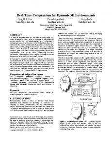
I. I NTRODUCTION URING the last years modern vision systems have made a big leap and reached impressive performance levels. Unfortunately this often entails a complex interaction of different vision tasks that put high computational demands. Recently, stereo camera based approaches have become very popular. Modern stereo matching algorithms are no longer sparse and feature-based but deliver a depth estimate for nearly every pixel of the image. Hirschmüller et al. [17] established a matching scheme called semi-global matching (SGM) that was made available on FPGA hardware by Gehrig et al. [14]. This low-power solution for matching stereo image pairs delivers dense disparity images in real-time. Such an exemplary disparity image encoding the depth information of the scene is shown in Figure 1a. The effort spent to traverse the disparity image in order to extract task-relevant information grows significantly with the rising variety of independent vision tasks. As a consequence, a lot of the scene content and object information is extracted repeatedly.

D

David Pfeiffer is employee of the Daimler AG, Sindelfingen/Germany and Ph.D. Student at the Humboldt-University of Berlin. e-mail: (see http://www2.informatik.hu-berlin.de/~dpfeiffe/). Uwe Franke is head of the Daimler AG research lab for mobile environment perception and image understanding in Sindelfingen/Germany.

(a)

(b)

Figure 1: Visualization of the SGM disparity image (a) and the extracted Stixel representation (b) for an urban traffic scenario. The color encoding is red for close and green for measurements far away.

This asks for a generic pre-processing step. By having a priori knowledge of the spatial arrangement of the 3D world, these different tasks could directly focus on their application specific domain. Thus, the available processing power can either be minimized or used in a more optimized fashion. This problem is addressed by introducing a medium level representation for three-dimensional objects. These are approximated by a set of rectangles called Stixels, all sharing the same width within the image (e.g. 5 px). Each Stixel describes the distance and height of an object in a certain image column. The space up to the base point of each Stixel is considered as free. Objects are idealized to stand on the ground with an approximately vertical pose. The set of all Stixels is called the Stixel World [3]. The Stixel World generated from the given disparity image is illustrated in Figure 1b. Since this representation describes three-dimensional information we also provide a virtual 3D view as shown in Figure 2. Literature holds a variety of different approaches to model objects in three-dimensional environments. A lot of them originate from the automotive or robotics domain and are either kept very simple or are not practicable in their usage. E.g. box shapes (3D and 2D) are frequently used in tracking processes for cars [5] or pedestrians [9], [21] but are rigid and thus not capable to follow the contour of complex objects precisely. Other representations, like free-form contours [7], polygons shapes [27] or level-sets [12] are not intuitive to handle. For automotive application Hu et al. [20] have discussed the benefits of the u-v-disparity space and presented an approach

2

Figure 2: 3D Stixel World representation of the urban scenario depicted in Figure 1. It is computed by using a stereo camera system only. Stixels approximate the boundaries of parked cars up to a depth of more than 35 m.

Figure 3: 3D dynamic Stixel World showing a person riding a bicycle. The color scheme symbolizes direction and speed of the dynamic Stixels, which are tracked independently. The arrows point into the moving direction of each Stixel.

to fit oriented planes to disparity maps, thus organizing the 3D environment in a structured way [20]. Sophisticated techniques have been introduced in order to detect and track the state of moving objects in non-explicit grid based representations. Gindele et al. [15] use a combination of a Bayesian occupancy filter with probabilistic velocity objects in order to generate a dynamic 4D map of the environment. Danescu et al. presented approaches for tracking multiple objects on behalf of the combination of particle filters with digital elevation maps or dynamic occupancy grids [8]. Further inspiration can be found in the domain of computer graphics. Unfortunately their objectives often differ from ours, e.g. the ease of access to either large or complex data sets (octtrees [29]) or to optimize the usage of limited system resources such as main memory. Coming from that domain Gallup et al. [13] have introduced an approach to approximate three-dimensional objects by a set of thin box volumes. Their principle turns out to be very similar to our Stixel objective. Even though all of these representations may be optimal for their application in each of their particular use cases, they do not match the criteria that we put on a 3D representation for dynamic environments. Some of them are either not explicit (e.g. grid based structures), require additional computational effort and are mathematically complex to manage or are not practical to be utilized for tracking purposes. Others do not balance the right level of abstraction and are thus either to fine, like point based models, or to coarse, such as box volumes or polygons. Hence, we consider the Stixel World to be a well suited medium level representation to decouple between low-level (pixel based) and high-level (object based) vision in the domain of mobile vision systems. By varying the width of the Stixels, the level of detail of the Stixel World can be chosen freely. In addition, this representation provides extraordinary robustness capabilities to outliers, missing stereo data or other disturbances. Furthermore it comes along with significant compression rates of the input data volume: Given a width of 5 px for the Stixels, the relevant content of a 1024 × 440 px disparity image can be described by 205 Stixels only. By introducing a tracking scheme similar to the principle of 6D-Vision [11], the Stixel Representation is extended into the

time domain [25]. As a result we gain access to velocity information for each Stixel independently. Consequently, we can distinguish between static and dynamic Stixels. An exemplary result for dynamic Stixels is depicted in Figure 3. It shows a bicyclist taking a left turn in front of our own vehicle. In this contribution we intend to give an introduction into the Stixel World. The article is organized as follows: Firstly, the building process of the Stixel World is sketched. Secondly, section III outlines the tracking process in order to gain access to information about the individual motion state of each Stixel. Section IV presents our experimental results for both static and dynamic Stixels. Further, section V incorporates the results of an analysis with a closer look into the range accuracy that can be achieved. Additionally, section VI sketches an exemplary automotive application that showed great benefit from using the Stixel World. Finally, section VII concludes this contribution. II. B UILDING THE S TIXEL W ORLD In the Stixel World each Stixel represents the first object encountered along a particular column of the image and thus encodes the distance, the location of the base point and the height of that object in 2D and 3D. The Stixel representation for a given situation is obtained in four steps: (1) generate a disparity image for the given stereo image pair, (2) determine the base points by computing the freespace using an occupancy grid, (3) perform a height segmentation to obtain the height of the objects and (4) extract the Stixel depth by using a histogram-based disparity registration scheme. A. Dense Stereo Stereo vision has been an active area of research for decades. For commercial stereo based products correlationbased approaches are popular, such like the driver assistant systems offered by Subaru or Toyota. Among the topperforming algorithms in the Middlebury database [28], we found semi-global matching (SGM) [17] to be the most efficient. Roughly speaking, SGM performs an energy minimization in a dynamic programming fashion on multiple 1D paths

3

Figure 4: Both figures illustrate a polar occupancy grid. Orange represents the likelihood for areas to be occupied, blue models the likelihood for street occurrence. The right grid is computed from the left one by applying the background subtraction. The green line corresponds to the freespace in polar coordinates obtained by dynamic programming.

crossing each pixel and thus approximates a 2D optimum. This energy consists of three parts: a data term for photoconsistency, a small smoothness energy term for slanted surfaces that change the disparity slightly, and a larger (constant) penalty term for depth discontinuities. Based on this algorithm, Gehrig et al. have introduced the first real-time dense stereo implementation using a Xilinx FPGA platform with a power consumption of less than 3 W [14]. For our purpose, we use a variant of that implementation which is able to compute 1024 × 440 px disparity images at a rate of 25 Hz. An exemplary disparity image for a common urban traffic scene is depicted in Figure 1a. B. Freespace Computation The freespace defines the space in front of that car, which can currently be passed without colliding with an obstacle. It is computed from an occupancy grid in three steps: Obtaining a polar occupancy grid, background subtraction and dynamic programming. Occupancy grids are commonly used to stochastically model the likelihood of the environment to be occupied [18], [22], [24]. Such grids are obtained by registering stereo disparities in their associated cells while considering the depth uncertainties known from the used stereo algorithm. The more stereo disparities are mapped to a cell, the higher is its likelihood to be occupied. Badino et al. have discussed several representations for occupancy grids in detail [2]. They found the polar column disparity grid (u, d) to be the most suitable to compute the freespace with. This is due to two unique properties of this representation. Firstly, an efficient search for freespace must be done in the direction of rays leaving the camera. In polar coordinates every grid column is, by definition, already in the direction of a ray. Secondly, it is straightforward to model disparity uncertainty taken from the stereo and triangulation uncertainty with respect to the camera geometry. In this representation these properties are incorporated by convolution with the same location-independent Gaussian kernel mask for every cell of the grid. An exemplary column disparity grid is depicted in Figure 4a. For a better understanding of the spatial context the grid from Figure 4a has been remapped to a Cartesian representation shown in Figure 5.

Figure 5: This Cartesian occupancy grid is obtained by a transformation of the polar grid given in Figure 4a. The freespace polygon is overlaid using a green coloring. Our car is centered at the bottom of the grid. Having such a polar representation, the task is to find the first visible relevant obstacle in the positive direction of depth. Looking at Figure 4a this means that the search must start from the bottom of the polar occupancy grid in vertical direction until an occupied cell is found. The space in front of that cell is considered as freespace. In a typical traffic scene, objects are found at multiple levels in a given column, leading to one foreground and multiple background objects. As an example note in Figure 1 that both the row of parking cars and the buildings in the background have a corresponding occupancy likelihood in the occupancy grid shown in Figure 4a and 5. In order to enforce the selection of the first obstacle, a background subtraction is carried out. All occupied cells behind the first maximum which are above a certain threshold are marked as free. This threshold must be selected dynamically in such a way that it is considerably larger than the expected noise in the occupancy grid. An example of the resulting grid is shown in Figure 4b. Every possible freespace solution is associated with a cost energy. Dynamic programming (DP) [6] is used to find the optimal path cutting the polar grid from left to right, while aiming for spatial and temporal smoothness. Both properties are required for reasons of robustness. Spatial smoothness is supposed to avoid dispensable jumps in depth while temporal smoothness models the expectation of the result to be similar to the result of the previous cycle. Every cell Cu,d0 of the polar occupancy grid is associated with costs for having Cu+1,d1 as a potential freespace neighbor. As typical for a global approach that cost consists of a data and a smoothness term and is defined by C (u, d0 , d1 ) = −L (u, d0 ) + Es (d0 , d1 )

(1)

where −L(u, d0 ) is the data term defined by the negative occupancy likelihood from the occupancy grid and Es (d0 , d1 ) = S (d0 , d1 ) + T (d0 , dˆ0 )

(2)

is a smoothness term containing a spatial and a temporal part. The spatial term penalizes jumps in depth and is defined as S (d0 , d1 ) =

Csf s

 ·

` (d0 , d1 ) , if ` (d0 , d1 ) < Ts . (3) Ts , if ` (d0 , d1 ) ≥ Ts

4

Figure 6: Visualization of the freespace result after applying dynamic programming to the polar occupancy grid from Figure 4b.

Figure 7: Visualization of the membership votes with white meaning positive (belonging to the object), gray neutral and black negative (background).

The function `(d0 , d1 ) returns the metric depth distance between the cells in rows d0 and d1 of the polar grid. The constant Csf s weights the costs for jumps in depth and the threshold Ts saturates this cost function, allowing the preservation of depth discontinuities. The temporal term has the same form:

Therefore, every disparity du,v votes for its membership to the foreground object located at (u, db ). In the simplest case a disparity votes positively for its membership as belonging to the foreground object if it does not deviate more than a maximum distance from the expected disparity db of the object, and negatively otherwise. Such a Boolean assignment makes the choice of the threshold very sensitive and does not consider the actual deviation of disparities. A smoother voting is achieved by means of an exponential function of the form

T (d0 , dˆ0 ) = Ctf s ·



`(d0 , dˆ0 ) , if `(d0 , dˆ0 ) < Tt , if `(d0 , dˆ0 ) ≥

Tt . (4) Tt

Hereby, Ctf s is the temporal cost parameter, Tt is the maximum distance for the saturation. The term dˆ0 is the disparity prediction of the freespace at the current row position which is obtained by applying an ego-motion correction to the freespace result of the previous cycle. For our results we use the freespace parameters Csf s = 2, Ts = 5 m, Ctf s = 0.001 and Tt = 5 m. Despite the small penalty Ctf s , the temporal smoothing provides robustness against missing or incomplete data (e.g. windshield wipers covering parts of the image). The output of the DP is a set of vector coordinates (u, db ), where u is a column of the image and db the disparity corresponding to the distance up to which freespace is available. Note that each freespace point (u, db ) of the occupancy grid shown in Figure 4b indicates not only the end of the freespace, but describes the location of the base-point of the first obstacle located at that position. That property is illustrated in Figure 6 where the freespace is projected into the left image. For every pair (u, db ) a coordinate (Xu , Zu ) is triangulated, which defines the corresponding 2D world point. The sorted collection of the points (Xu , Zu ) plus the origin (0, 0) form a polygon which defines the freespace area in Cartesian coordinates from the camera’s point of view (see Figure 5). The next section describes how to apply a second pass of dynamic programming in order to obtain the upper boundaries of the objects. C. Height Segmentation The height of the objects which limit the freespace is obtained by finding the optimum segmentation between foreground and background disparities. This is achieved by first computing a cost image from the disparity image and by then applying dynamic programming to find the upper boundary. Given the set of freespace points (u, db ) and their corresponding triangulated Cartesian coordinates (Xu , Zu ) obtained in the previous step, the task is to find the optimum row position vt where the upper boundary of the object at (Xu , Zu ) is located.



M (u, v) = m (du,v ) = 2

1−

 (d

u,v −db ) ∆Du

2 

− 1.

(5)

The term ∆Du is a computed parameter that is derived for every column u independently via ∆Du = db − fd (Zu + ∆Z) ,

(6)

where the function fd (Z) computes the disparity corresponding to depth Z. This approach has the objective to define the membership as a function in meters instead of pixels to take perspective effects into account. For the shown results we use ∆Z = 2 m. Since all objects must have a positive height only rows above the image coordinate (u, vb ) have to be considered, where vb is the row position of the base point (Xu , Zu ). Figure 7 shows the resulting membership votes for our exemplary scene. From these membership votes a cost image is computed via vb v−1 X X C (u, v) = M (u, f ) − M (u, b) . (7) f =v

b=0

Note that the origin (0, 0) of the image coordinates is assumed in the top left corner. Equation 7 expresses the idea that the maximum Cumax (and thus the highest likelihood for the height segmentation to perform a cut in column u) is supposed to be reached at row vumax when most positive membership votes lie below (foreground) and the most negative membership votes lie above vumax (background). Figure 8 shows the resulting costs when this method is applied to the membership votes illustrated in Figure 7. For the computation of the optimum path every row v0 of a column u is associated with a cost for having row v1 in column u+1 as its possible neighbor. This is very similar to the cost term defined in Section II-B. The cost for every possible segmentation between two neighbored columns is composed of a data and a smoothness term: C (u, v0 , v1 ) = −C (u, v0 ) + Su (u, v0 , v1 ) ,

(8)

5

σd = 0.4 px. A parabolic fit around the maximum found in the histogram delivers the new and more precise sub-pixel depth information. In addition, this approach offers outlier rejection and noise suppression of the raw SGM input. Figure 8: Visualization of the cost image (data term) used for the dynamic programming in the height segmentation. Bright values represent a high likelihood to perform the foregroundbackground cut.

III. T HE DYNAMIC S TIXEL W ORLD The precision of the static Stixel World can be improved further if temporal dependencies between consecutive images are taken into account. In addition, tracking Stixels allows to reveal the motion of dynamic objects within the scene. Estimating the absolute motion states of other objects requires knowledge of the ego-motion. Consequently, we extend the idea of the static Stixel World to the time domain. A. The 6D-Vision Principle

Figure 9: Result of the height segmentation after applying dynamic programming. The yellow line indicates the segmentation of foreground and background.

where the cost image C(u, v) is used as the data term and S(u, v0 , v1 ) is a smoothness constraint that penalizes jumps in the vertical direction. The smoothness term is defined as: S (u, v0 , v1 )

= ·

Cshs · |v0 − v1 |   |Zu − Zu+1 | max 0, 1 − NZ

(9)

The smoothness costs S(u, v0 , v1 ) for a jump in height is proportional to the difference between the rows v0 and v1 with Cshs as a constant penalty factor. The distances Zu and Zu+1 correspond to the freespace coordinates (u, db ) and (u+1, db ). The right term of the product has the effect of relaxing the smoothness constraint at depth discontinuities and becomes zero if the difference in depth between adjacent columns is equal or larger than NZ . In this case these columns are assumed to belong to different objects and thus we must not demand smoothness of the height. Our results for the height segmentation are generated using NZ = 5 m and Cshs = 8. The segmentation result for our exemplary scene corresponding to the freespace shown in Figure 6 is depicted in Figure 9. D. Stixel Extraction Once the freespace and the height for every column has been computed, the extraction of the static Stixels is straightforward. The properties base and top point vb and vt as well as the width of the Stixel span a rectangle where the Stixel is located within the image. Since the occupancy grids are discretized to equidistant steps in disparities, the freespace vector inherits this finite resolution and is thus limited in precision. To overcome this limitation the depth for each Stixel is refined. All disparities found within a Stixel are registered in a histogram while regarding the depth uncertainty known from SGM . The SGM disparity error is assumed to be normally distributed with

Franke et al. presented a method called 6D-Vision [11] that allows for the simultaneous estimation of 3D-position and 3D-motion for a large number of 2D point features. These features are tracked over time by using Kalman filters [31] resulting in a rich 6D representation that combines position ˙ Y˙ , Z) ˙ T for and velocity in the state vector X = (X, Y, Z, X, every feature independently. The underlying motion model is to have a constant velocity with v˙ = a = 0. For our tracking purpose, we follow this principle with the additional restriction of Y˙ = 0, since we do not expect the Stixels to move vertically. Therefore, our state vector is reduced to 4D and only the position and velocity consisting ˙ Z) ˙ T have to be estimated. of X = (xT , v T )T = (X, Z, X, For scenarios with severe gradients of the road surface that approximation results in small errors of the velocity estimate. However, that is regarded negligible for our purpose. B. Ego-motion Estimation In order to estimate the absolute motion states of the Stixels, the motion of the ego vehicle must be known. Certainly, this information can be taken from inertial sensors. However, we prefer to use the method described in [1] since it outperforms available standard inertial sensors with respect to precision. The basic idea of this approach is to track static image points over time and use their depth to estimate the motion with full six degrees of freedom. The optimal 3D translation and 3D rotation between consecutive images is determined in a least square error minimization approach. In order to reduce drift errors, multi-frame estimations of the resulting poses are performed. C. Motion Estimation for Dynamic Stixels Assuming a constant velocity vc and a constant yaw rate ψ˙ c for a given time interval ∆t = tk − tk−1 , the movement of a vehicle can be described in that car’s right-handed coordinate system by   ˆ ∆t vc 1 − cos ψ˙ c ∆t v c (τ )dτ = . (10) ∆xc = sin ψ˙ c ∆t ψ˙ c 0

6

The new position of a world point located at xk = (X, Z)Tk after the time interval ∆t is described by xk = Ry (ψc )(xk−1 + v k−1 ∆t − ∆xc ).

(11)

Having a filter position xk−1 = (X, Z)Tk−1 and an estimated ˙ Z) ˙ T velocity v k−1 = (X, k−1 for a Stixel, the system and measurement model of the extended Kalman filter is deduced. The system model is given by X k = Ak X k−1 + B k + ω k .

(12)

With  Ak

Bk

=

=

 Ry (ψc ) ∆tRy (ψc ) 02×2 Ry (ψc )   1 − cos ψ˙ c ∆t  ˙ 1   − sin ψc ∆t  .   0 ψ˙ c 0

(13)

Ry corresponds to the 2 × 2 rotational matrix revolving around the y-axis. The noise vector ω k is assumed to be Gaussian white noise with covariance matrix Q. Since we operate on rectified images, the pin-hole camera model applies by using the non-linear measurement equation     u Xfu 1 z =  v  =  Y fv  + γ (14) Z d bfu with the focal lengths fu and fv and the baseline b of the stereo camera system. The noise vector γ is assumed to be Gaussian white noise with a covariance matrix R. This non-linear projection from our system state to the measurements requires to use an extended Kalman filter. The resulting measurementstate-relation for the Kalman filter is obtained by the Jacobian approximation of equation (14). A measurement to update the Kalman filter and the height property of a tracked Stixel at time-step k consists of three , the disparity parts: The new image coordinate (u, v)meas k and a height observation hmeas . measurement dmeas k k Thus, in addition to stereo, an algorithm to measure the 2D Stixel motion between two consecutive images is required. For this purpose, we rely on the dense optical flow method as introduced by Zach et al. [32] that is based upon the variational approach of Horn and Schunk [19]. However, any other optical flow algorithm (preferably offering sub-pixel accuracy) serves the purpose just as well. The coordinate measurement (u, v)meas for the new area Ωk k of the Stixel within the current image is computed from the optical flow vectors Uk−1,k within its previous area Ωk−1 . Then, the area Ωk is used to compute the new disparity measurement dmeas from the current disparity image Dk . This k procedure is mathematically described with the following equation: (u, v)meas k dmeas k

=

(u, v)meas k−1 + ∆u (Uk−1,k , Ωk−1 )

= d (Dk , Ωk )

(15)

The function ∆u(Uk−1,k , Ωk−1 ) computes the displacement for Ωk−1 from the optical flow image Uk−1,k . The function d(Dk , Ωk ) is the equivalent of ∆u(. . .) with respect to the disparity image Dk and the area Ωk . Further, we consider scaling effects due to changes of depth as insignificant for our measurement generation. Generally, the height of each Stixel is assumed to remain constant. However, when approaching an object, the quality of the height measurement for a Stixel representing that object tends to increase and additionally updating the height property of that Stixel is reasonable. Therefore, the closest static Stixel is determined and its height is adopted. As a result no additional height segmentation for the dynamic Stixels is required. The height information is updated by means of a low pass filter via hmeas k

=

hstatic

hk

=

α · hk−1 + (1 − α) · hmeas k

(16)

with α ≈ 0.95 as a fixed and rather insensitive parameter. The initialization process for the Kalman filter motion state exploits already existing Stixels for a neighborhood initialization. Qualified neighbors have to fulfill certain fitness criteria, such as a minimum age and a maximum normalized innovation squared (NIS). The NIS is the Mahalanobis distance between the predicted and the actual measurements [4]. The motion states are fused according to their particular filter state variances. When no qualified neighbors are available the tracker uses a multi-filter approach for faster convergence [11]. For this purpose, multiple hypothesis are used, one for each moving direction along the X and Z-axes plus a static one. For performance reasons the filter system is reduced to a single filter after 15 update steps. Hence, the filter with the smallest NIS is chosen. Due to the possible lateral movement, dynamic Stixels are no longer bound to equidistant columns. Consequently, the total number of dynamic Stixels is not fixed. They start to overlap partially or can belong to objects in different depths. Converged Stixels are detected as twins and merged according to the variances of their Kalman filters, such that their total maximum number does not increase exorbitantly. Depending on the actual parameters, a scene is described with up to two times as much dynamic as static Stixels. IV. E XPERIMENTAL R ESULTS The depicted video material has been recorded in our test vehicle using an 1024 × 440 imager with a 42° lens and a focal length of 1273 px. The baseline of the stereo rack is approximately 22 cm. The SGM stereo matching is running asynchronously on an FPGA (Xilinx Virtex-4) within 40 ms causing one frame delay. The dense optical flow is calculated on the GPU (NVidia 285GTX) using a CUDA implementation that takes roughly 35 ms to compute. This step is performed asynchronously as well. The remaining algorithm is running on the CPU (Core i7-980X 3.33Ghz, 6GB DDR3 1333) in real-time within ∼ 30 ms. This time splits as follows: • rectification of the images: less than 2 ms

7

Z

5m/s

-5m/s

5m/s

X

-5m/s

Figure 13: The circle illustrates the color encoding of speed and direction. Maximum saturation is reached with 10 m/s. The color value represents the direction the Stixel moves with respect to our ego-vehicle that is in line with the Z-axis.

• • • •

freespace computation: 10 ms - 4 ms for the depth map, 5 ms for the dynamic programming step height segmentation: 11 ms - 3 ms for the cost image, 8 ms for the dynamic programming step static Stixel measurements: 2 ms (including distance refinement with histogram based approach) dynamic Stixels: 3 ms. Note that this is a mean value. It depends on the actual number of tracked Stixels.

Figure 14: Visual comparison of the stereo result from SGM (top) against a non-artificial ground truth (bottom) obtained from the LIDAR Velodyne HDL-64E.

algorithm was successfully evaluated in our test vehicle for hours of open road traffic. The Kalman filters used for these results estimate position and velocity for every Stixel independently. Depending on the filter configuration a reliable motion estimate is available within 3 update steps. To obtain further state information such as acceleration these filters can be extended accordingly. V. E VALUATION U SING R EFERENCE S ENSORS

A. Result of the Static Stixel World The images depicted in Figure 10 show a couple of situations and their corresponding static Stixel representations. These include urban environments as well as humans at close range. More examples for static Stixels including further scenarios such as highways or rural roads can be found in [3]. Note how the Stixel representation is able to follow the contour of the objects and thus approximates those very precisely. For all images in the following exemplary illustrations a Stixel width of 5 px has been chosen. Varying this parameter grants the freedom to determine the trade-off between compactness and the level of detail of the approximation. The Stixel extraction scheme proves to be quite robust. All examples have been generated with the same set of parameters. No additional parameter tuning was performed. B. Results of the Dynamic Stixel World The depicted images shown in Figure 11 illustrate basic examples by featuring only a few moving objects. Additional scenarios are presented in Figure 12. These include 3D-views and correspond to more complex traffic situations with either several moving objects, a higher egomotion or even non-rigid motion of the objects themselves. The coloring for the dynamic Stixels encodes the movement along the XZ plane and is explained together with our vehicle coordinate system in Figure 13. A short explanation regarding the motivation for each scene as well as a description of contents is given below each illustration. Even though these are just exemplary, the Stixel

The reliability of the Stixel World is directly dependent on the quality of the original stereo data. By relying on semiglobal matching [17] for the stereo computation we chose one of the top-performing algorithms found in the Middlebury database [28]. Even though this database is a good platform to compare and rank stereo matching algorithms under controlled environmental conditions, detailed surveys on the accuracy and reliability of stereo algorithms in real-world and automotive scenarios are still an open topic [23], [30]. When dealing with safety and assistance systems for automotive application, awareness of such properties becomes mandatory. For this reason we had a closer look into the range accuracy that can be achieved when using the Stixel World to represent the three-dimensional environment [26]. Consequently, we evaluated our algorithms against a reference sensor and thus decided to use the Velodyne HDL-64E [16]. That 360° LIDAR was widely used in the DARPA Urban Challenge. Due to its depth-independent measurement noise it is very well suited for this task. It was used to generate virtual disparity images that serve as non-artificial ground truth. An exemplary visual comparison between the SGM based disparity image from Figure 1a and a LIDAR based disparity image for the same urban scenario can be seen in Figure 14. For the evaluation two sets of scenarios were chosen: One is well arranged showing industrial containers at several distances. It exhibits no slanted or reflecting surfaces, puddles or windows. The other one is a more practical urban environment as depicted in Figure 14. As it turns out for the urban scenario, the Stixel representation yields remarkable range accuracy of less than 0.4 m deviation at a distance of 30 m. The plot

8

(a) Urban scenario with a leading car, buildings on the right and an oncoming car on the left side of the road.

(b) Crowded urban scenario with a leading car, several cars on the left, houses and pedestrians on the right side.

(c) A person and various other objects are located ahead at different depths.

Figure 10: A set of exemplary scenarios are illustrated together with their corresponding static Stixel representation. The colors of the Stixels encode the distance with red representing close and green representing far objects.

(a) A car is moving from left to right. Its estimate velocity is ≈ 12 m/s. Parking vehicles and the infrastructure are correctly estimated as standing still.

(b) A car is moving away from us with an estimated speed of ≈ 9 m/s. Note how the drawn arrows are aligned in parallel and thus point into the same direction.

(c) An approaching car takes a left turn ahead of us. Stixels on its front correctly point into that direction.

Figure 11: Four different exemplary scenes are illustrated showing rather clearly arranged traffic scenes with only a few moving obstacles. The sequences within the parking site were taken while standing still. Where Stixels are estimated as moving, arrows are drawn that point into the direction where they are expected within the next half second.

Figure 15: Evaluation of the Stixel World by using a high performance LIDAR. The black curve denotes the deviation of Stixels compared to the LIDAR (as a function of the distance), blue shows the corresponding standard deviation of the Stixels and red denotes the average standard deviation of the LIDAR measurements withing the region of a Stixel itself.

presenting the test results for the urban scenarios is given in Figure 15. The black graph marks the deviation of Stixels compared to the distance measurement of the LIDAR. It is slightly growing with an increasing distance, from a few centimeters at 15 m

range to about 0.4 m at 30 m. The blue curve denotes the standard deviation of that difference while the red curve represents the average standard deviation of LIDAR measurements within the area Ω of each Stixel. Since we compare the Stixels to the LIDAR, that red curve has to be a lower bound for the blue one. With that in mind, we consider the experimentally shown quality of the Stixel World as outstanding, especially for a stereo based representation that is reconstructed purely from a single stereo image pair. Anyhow, this evaluation made a handful of further insights apparent. Besides revealing how crucial it is to have a flawless sensor calibration, applying this method also allowed us to identify (and correct) even slight calibration errors within the magnitude of 0.01°, as e.g. within the squint angle calibration of our stereo camera system. The complete and more detailed evaluation can be found in [26]. VI. A PPLICATION OF THE S TIXEL W ORLD The Stixel World is well suited as a medium level representation to decouple low-level data from high-level algorithms. It corresponds to a figure-ground segmentation that offers a precise contour approximation. By varying the width of the Stixels, the user can individually choose between the compactness and the detail of the medium level representation. Given a 1024 × 440 px image and a fixed width of 5 px for the Stixels, the whole scene is described in 205 Stixels, while

9

(a) This figure illustrates a common traffic scene within an urban environment, containing both static and moving objects. Our vehicle speed equals 8 m/s. One can see the walls aside standing still (white coloring) while the three cars (one in front and two on our left side) move along our direction (blue). At a distance of ≈ 35 m a fourth car on an approaching lane is visible. Its heading direction is roughly estimated correctly contrary to our movement.

(b) A view on an intersection is illustrated within this figure. A truck is moving in from the left and turning to its left. The performed rotation is made visible by the different colors of the Stixels covering the truck, since the rear moves differently from the front.

(c) A car is moving from right to left and performs a left turn at an intersection. It moves rather rigidly with an approximate velocity of 12 m/s, as denoted by the uniform orange coloring.

Figure 12: More complex results of dynamic Stixels are shown. The color encoding is explained in Figure 13. To be able to illustrate the motion properties and spatial alignment in detail, 3D-views of the scene are given besides the pictures.

every Stixel is defined by 2 parameters only (distance and height). The lateral position is given by the ordering, thus the set of Stixels additionally encodes the freespace available to maneuver. In total we achieve a reduction of the data volume of 99.9%: more than 450000 disparity measurements reduced to 410 values. The extraction scheme proves to be robust against outliers in the input data. With minor changes of the input data between two consecutive frames this representation is still alike. In contrast to tree-based structures or graphs it does not require complex reorganization. Furthermore, the Stixel representation is predestined to be grouped to objects due to their spatial vicinity as shown in Figure 16. Thus, it is very suitable for tasks like control of attention, object detection and object tracking as done in the work of Barth et al. [5]. In their framework Stixels are grouped

to clusters by using straightforward heuristic techniques. The spatial orientation and silhouette of these groups is used as a prior and a constraint within a vehicle tracking approach. The L-shape that is typical for a group of Stixels representing a vehicle is utilized to improve the orientation estimate of the tracked vehicles. The tracker of Bart et al. [5] is a feature based point tracker. Thus, the silhouette of the Stixel representation for the car is used to decide whether tracked points should be assigned to the car or if they should be disregarded. Exemplary results of their method are depicted in Figure 16. Erbs et al. [10] proposed an approach with the objective to group Stixels to objects in order to detect whether those are moving or belong to stationary background. Their probabilistic segmentation scheme performs an energy minimization that guarantees to obtain the optimum segmentation using a priori knowledge as well as geometrical information about the three-

10

team for mobile perception (GR/PAP) of the Daimler AG in Sindelfingen. Without the dedicated effort of the colleagues, several aspects of the presented work could not have been realized. Especially, we feel indebted to thank Stefan Gehrig and Clemens Rabe for their fruitful as well as inspiring discussions and their unreserved support. Special thanks are due to Alexander Barth for providing material of his experimental results when adapting his algorithms in order to incorporate the Stixel World in his vehicle tracking framework. Figure 16: Application of Stixels in a vehicle tracking system. The color bands at the bottom mark groups of Stixels, the boxes around the cars show their estimate orientation and the green “carpet” illustrates the predicted trajectory of the vehicle. The estimate of the orange boxes utilizes the orientation of grouped Stixel clusters. dimensional scene. VII. S UMMARY AND C ONCLUSION With the Stixel World we present a medium level representation to model the freespace and obstacles of the threedimensional environment in a very compact and robust manner. Stixels allow to achieve significant compression rates compared to the raw input that is generated from dense stereo and optical flow computation. Furthermore, they independently provide the world motion of the objects. Dense disparity images are used to compute cost images for the freespace computation and the height segmentation. Dynamic programming is applied to these cost images to ensure spatial and temporal smoothness of the results. This information is used to extract the static Stixel World. Motion information is derived from tracking dynamic Stixels over time by means of Kalman filters and the use of optical flow. By relying on a high performance LIDAR as reference sensor we have been able to warrant this representation an outstanding accuracy performance. Its direct and straightforward application into the work of Barth et al. renders the true potential this representation has for future vision based applications. Especially with an increasing variety of independent vision tasks, having such a prior knowledge of the three-dimensional scene arrangement will become more and more indispensable. In conjunction with the motion information, dynamic Stixels form a powerful medium level representation to support further processing steps such as object clustering, control of attention and reasoning. The estimation of motion works very precisely and thus delivers reliable and easy to access state information. Experimental results show the robustness of our real-time capable method. The Stixel World is not limited to an application in driver assistance tasks only, but is easily extended to be of use in various other domains such as augmented reality, GIS or robotics. ACKNOWLEDGMENT The presented work is far from being an individual achievement, but the result of a very successful collaboration of the

R EFERENCES [1] Hernán Badino. A robust approach for ego-motion estimation using a mobile stereo platform. In 1st International Workshop on Complex Motion, IWCM, Günzburg, Germany, October 2004. Springer. [2] Hernán Badino, Uwe Franke, and Rolf Mester. Free space computation using stochastic occupancy grids and dynamic programming. In Workshop on Dynamical Vision, ICCV, Rio de Janeiro, Brazil, October 2007. [3] Hernán Badino, Uwe Franke, and David Pfeiffer. The Stixel World - A compact medium level representation of the 3D-world. In German Association for Pattern Recognition (DAGM), pages 51–60, Jena, Germany, September 2009. [4] Yaakov Bar-Shalom, Thiagalingam Kirubarajan, and X.-Rong Li. Estimation with Applications to Tracking and Navigation. John Wiley & Sons, Inc., New York, NY, USA, 2002. [5] Alexander Barth, David Pfeiffer, and Uwe Franke. Vehicle tracking at urban intersections using dense stereo. In 3rd Workshop on Behaviour Monitoring and Interpretation, BMI, pages 47–58, Ghent, Belgium, November 2009. [6] Richard Bellman. Dynamic Programming. Princeton University Press, 1957. [7] Thomas Brox, Bodo Rosenhahn, and Joachim Weickert. Threedimensional shape knowledge for joint image segmentation and pose estimation. In German Association for Pattern Recognition (DAGM), pages 109–116, Vienna, Austria, September 2005. [8] Radu Danescu, Florian Oniga, and Sergiu Nedevschi. Particle grid tracking system for stereovision based environment perception. In IEEE Intelligent Vehicles Symposium (IV), pages 987–992, San Diego, CA, USA, June 2010. [9] Markus Enzweiler and Dariu Gavrila. Monocular pedestrian detection: Survey and experiments. IEEE Transactions on Pattern Analysis and Machine Intelligence (PAMI), 31(12):2179–2195, 2009. [10] Friedrich Erbs, Alexander Barth, and Uwe Franke. Moving vehicle detection by optimal segmentation of the dynamic Stixel World. In IEEE Intelligent Vehicles Symposium (IV), pages 951–956, Baden-Baden, Germany, June 2011. [11] Uwe Franke, Clemens Rabe, Hernán Badino, and Stefan Gehrig. 6dvision: Fusion of stereo and motion for robust environment perception. In German Association for Pattern Recognition (DAGM), Vienna, Austria, September 2005. [12] Michael Fussenegger, Rachid Deriche, and Axel Pinz. Multiregion level set tracking with transformation invariant shape priors. In Asien Conferenceon Computer Vision (ACCV), pages I:674–683, 2006. [13] David Gallup, Marc Pollefeys, and Jan-Michael Frahm. 3d reconstruction using an n-layer heightmap. In German Association for Pattern Recognition (DAGM), pages 1–10, Darmstadt, Germany, September 2010. [14] Stefan Gehrig, Felix Eberli, and Thomas Meyer. A real-time lowpower stereo vision engine using semi-global matching. In International Conference on Computer Vision Systems (ICVS), 2009. [15] Tobias Gindele, Sebastian Brechtel, Joachim Schröder, and Rüdiger Dillmann. Bayesian occupancy grid filter for dynamic environments using prior map knowledge. In IEEE Intelligent Vehicles Symposium (IV), 2009. [16] Velodyne Headquarters. High Definition Lidar HDL-64E S2. http:// www.velodyne.com/lidar/, February 2010. [17] Heiko Hirschmüller. Accurate and efficient stereo processing by semiglobal matching and mutual information. In IEEE Conference on Computer Vision and Pattern Recognition (CVPR), pages 807–814, San Diego, CA, USA, June 2005.

11

[18] Florian Homm, Nico Kaempchen, Jeff Ota, and Darius Burschka. Efficient occupancy grid computation on the gpu with lidar and radar for road boundary detection. In IEEE Intelligent Vehicles Symposium (IV), pages 1006–1013, San Diego, CA, USA, June 2010. [19] Berthold K. P. Horn and B. G. Schunk. Determining optical flow. In Artificial Intelligence, volume 17, pages 185–203, 1981. [20] Zhencheng Hu and Keiichi Uchimura. U-v-disparity: An efficient algorithm for stereovision based scene analysis. In IEEE 3D Digital Imaging and Modeling, pages 48–54, 2005. [21] Bastian Leibe, Konrad Schindler, Nico Cornelis, and Luc J. Van Gool. Coupled object detection and tracking from static cameras and moving vehicles. IEEE Transactions on Pattern Analysis and Machine Intelligence (PAMI), 30(10):1683–1698, 2008. [22] Larry Matthies and Alberto E. Elfes. Integration of sonar and stereo range data using a grid-based representation. In IEEE International Conference on Robotics and Automation (ICRA), volume 2, pages 727– 733, April 1988. [23] Sandino Morales, Tobi Vaudrey, and Reinhard Klette. Robustness evaluation of stereo algorithms on long stereo sequences. In IEEE Intelligent Vehicles Symposium (IV), pages 347 – 352, 2009. [24] Y. Negishi, J. Miura, and Y. Shirai. Vision-based mobile robot speed control using a probabilistic occupancy map. In Multisensor Fusion and Integration for Intelligent Systems, pages 64–69, August 2003. [25] David Pfeiffer and Uwe Franke. Efficient representation of traffic scenes by means of dynamic Stixels. In IEEE Intelligent Vehicles Symposium (IV), pages 217–224, San Diego, CA, USA, June 2010. [26] David Pfeiffer, Sandino Morales, Alexander Barth, and Uwe Franke. Ground truth evaluation of the Stixel representation using laser scanners. In IEEE Conference on Intelligent Transportation Systems (ITSC), Maideira Island, Portugal, September 2010. [27] Hong-Keat Pong and Tat-Jen Cham. Object detection using a cascade of 3d models. In IEEE Conference on Computer Vision and Pattern Recognition (CVPR), pages 808–811, New York, NY, USA, September 2006. [28] Daniel Scharstein and Richard Szeliski. Middlebury online stereo evaluation, 2002. http://vision.middlebury.edu/stereo. [29] Matthias Schmid, Mirko Maehlisch, Jürgen Dickmann, and HansJoachim Wuensche. Dynamic level of detail 3d occupancy grids for automotive use. In IEEE Intelligent Vehicles Symposium (IV), pages 269–274, San Diego, CA, USA, June 2010. [30] Pascal Steingrube, Stefan Gehrig, and Uwe Franke. Performance evaluation of stereo algorithms for automotive applications. In International Conference on Computer Vision Systems (ICVS), pages 285–294, Berlin, Heidelberg, 2009. Springer-Verlag. [31] Greg Welch and Gary Bishop. An introduction to the kalman filter. Technical report, Department of Computer Science, University of North Carolina at Chapel Hill, 1995.

[32] Christopher Zach, Thomas Pock, and Horst Bischof. A duality based approach for realtime tv-l1 optical flow. In German Association for Pattern Recognition (DAGM), pages 214–223, Heidelberg, Germany, September 2007.

Dipl.-Inf. David Pfeiffer The author David Pfeiffer studied computer science and received his diploma at the Humboldt-University of Berlin. The supervisor for his diploma thesis was Prof. Dr. rer. nat. Ralf Reulke. In addition, he worked for Prof. Reulke as a research assistant at the German Aerospace Center (DLR) for several years. Today, David is working towards his Ph.D. in computer science. For this purpose, he is employed at the Daimler AG in Sindelfingen, Germany where he elaborates his thesis as a member of the team GR/PAP lead by Dr. Uwe Franke. His area of research is the modeling of dynamic 3D environments by using stereo camera systems. His supervisor at the university remains Prof. Reulke.

Dr.-Ing. Uwe Franke Uwe Franke received the Ph.D. degree in electrical engineering from the Technical University of Aachen, Germany, in 1988 for his work on content based image coding. Since 1989 he has been with Daimler Research and Development and has been constantly working on the development of vision based driver assistance systems. He developed Daimler’s lane departure warning system (“Spurassistent”, available since 2000). Since 2000 he has been head of Daimler’s Image Understanding Group and is a well known expert in real-time stereo vision and optical flow. Recent work is on optimal fusion of stereo and motion, called 6D-Vision and scene flow. In 2002, he was program chair of the IEEE Intelligent Vehicles Conference in Versailles, France.