Proceedings of the 2009 Winter Simulation Conference. M. D. Rossetti ... These new models use an endogenous representation of individual agents together ...
Proceedings of the 2009 Winter Simulation Conference M. D. Rossetti, R. R. Hill, B. Johansson, A. Dunkin, and R. G. Ingalls, eds.
MODELING INTERACTION BETWEEN INDIVIDUALS, SOCIAL NETWORKS AND PUBLIC POLICY TO SUPPORT PUBLIC HEALTH EPIDEMIOLOGY Keith R. Bisset Xizhou Feng
Madhav Marathe Virginia Bioinformatics Institute and Department of Computer Science Virginia State University and Polytechnic Institute Blacksburg, VA, 24061 USA
Virginia Bioinformatics Institute Virginia State University and Polytechnic Institute Blacksburg, VA, 24061 USA
Shrirang Yardi Nvidia 2701 San Tomas Expressway Santa Clara, CA 95050 ABSTRACT Human behavior, social networks, and civil infrastructure are closely intertwined. Understanding their co-evolution is critical for designing public policies. Human behaviors and day-to-day activities of individuals create dense social interactions that provide a perfect fabric for fast disease propagation. Conversely, people’s behavior in response to public policies and their perception of the crisis can dramatically alter normally stable social interactions. Effective planning and response strategies must take these complicated interactions into account. The basic problem can be modeled as a coupled co-evolving graph dynamical system and can also be viewed as partially observable Markov decision process. As a way to overcome the computational hurdles, we describe an High Performance Computing oriented computer simulation to study this class of problems. Our method provides a novel way to study the co-evolution of human behavior and disease dynamics in very large, realistic social networks with over 100 Million nodes and 6 Billion edges. 1
INTRODUCTION
Pandemic diseases such as avian influenza are extremely serious threats to global public health security. Although public health authorities around the world are far more prepared to respond such threats than they have been in the past, a number of modern trends continue to make this a vexing problem. These include: (i) a larger global population and increased urbanization leading to a higher density of individuals within cities; (ii) higher levels of long distance travel, including international travel; (iii) increased numbers of elderly individuals and individuals with chronic medical conditions. Over the past several years, large-scale, individual-based, disaggregate models have been studied (Eubank 2002, Eubank et al. 2004, Halloran et al. 2008, Carley et al. 2006). These new models use an endogenous representation of individual agents together with explicit interactions between these agents to generate and capture the disease spread across social networks. In this paper, we describe an interaction-based highly resolved modeling approach for representing and reasoning about large scale epidemics. We build on our earlier work (Barrett et al. 2008), wherein we described EpiSimdemics– an interaction based high performance computing oriented simulation for studying large scale epidemics. We describe programming abstractions and models that allow us to extend EpiSimdemics to better reason about real-world situations. Specifically, we developed Simdemics, that in conjunction with EpiSimdemics, allows us to study the joint evolution of policy, disease dynamics, human behavior and social networks as an epidemic progresses. In classical models used in computational epidemiology, individuals do not change their contact behavior during epidemics. For example, they do not engage in social distancing during periods of high disease prevalence. Instead, they continue with their normal contacts (often modeled as uniform mixing) as if no epidemic were under way. Although potentially a reasonable assumption for non-lethal infections such as the common cold, it is known to be incorrect for lethal diseases such as AIDS. People adapt their contact patterns when they perceive a potential threat due to the onset of avian influenza. This will likely result in substantial changes in the social networks that in turn will alter epidemic dynamics. In other words, individual behaviors and
978-1-4244-5771-7/09/$26.00 ©2009 IEEE
2020
Bisset, Feng, Marathe, and Yardi the social contact networks that they generate interact and co-evolve. For brevity we will call the problem of co-evolution of Public policy, Individual behavior and interaction Network as the PIN problem for the rest of this section. Policy planning has been one of the central foci of epidemiological research over the years. In addition to empirical observations, practitioners have relied on mathematical models for understanding and comparing different public health policies and making recommendations. These models involve stochastic disease processes on social contact networks. Due to computational considerations, most work in epidemiological modeling has focused on static social networks. However, social networks change quite a bit during an epidemic. For instance, policies put in place by public health authorities such as school closures, quarantine, and face masks cause significant changes to the social network. Equally important, though, is the role of individual behavior in transforming the social network. The 2003 SARS epidemic serves as an excellent example of how both these factors changed the social network (Smith 2006). Thus, mathematical methods for analyzing epidemics based on models of static social contact networks are unlikely to give practical insights into the spread of diseases. We illustrate this by an example. Example. An important decision faced by millions of people throughout the country every day during cold and flu season: Should I go to work today, even though I have symptoms of a cold or flu? The immediate economic impact of absenteeism due to colds and influenza in the United States in 1980 is estimated to have been $6.5 Billion (Stewart et al. 2003). While some fraction of these infections arise from exposure outside the workplace, many – perhaps the majority – occur because a co-worker decided the consequences of possibly transmitting the disease were less important than the certain consequences of staying home. Indeed, the term presenteeism has been coined to describe the problem. We examine the factors involved in this decision more closely. Society pressures us in many ways to go to work even when we may be sick: lack of paid sick leave, the need to complete tasks, fear of being seen as a malingerer, desire to be perceived as critical to an organization’s success, etc. Personal interactions with co-workers can influence the decision in either direction. The influence co-workers exert may be tied to whether they have themselves been sick. Furthermore, when a person chooses to stay home, it affects the social network at work in at least two different ways: one is simply the removal of the sick person as an active influence in decision-making (note that this biases the influence of the remaining people by removing precisely those who would argue for staying home); the other, more subtle, effect is a change in the probability that co-workers will be infected, and thus a possible change in their influence on the decision. See (Epstein et al. 2007) for a discussion of the coupling of fear and disease. The factors in these example decisions – uncertain consequences, information about disease prevalence and conflicting motivations between micro and macro levels for individuals – are at the heart of issues such as non-compliance with public policy and, more generally, breakdown of the rule of law in society. The examples, though complex, are amenable to analysis using our Simdemics framework. 2
RELATED WORK
To study how infectious diseases spread through populations, epidemiologists have been using three major computational approaches: compartmental models, network-based percolation models, and agent-based models. Though the first two models are quite efficient from a computation standpoint, they either use unrealistic assumptions (e.g., compartmental models assumes the population is fully mixed and any susceptible individual has a uniform probability to be infected by any infectious individual) or can not provide information that is critical to epidemic planning and control (e.g., percolation models only yield the final outbreak size but give little time varying information about disease dynamics). As a relatively new approach, agent-based models are more powerful and realistic in describing the dynamics of disease spread, the impacts of population dynamics, and the effectiveness of complex interventions. Among many agent-based simulation methods, EpiSimdemics is closest to the simulation systems developed by Eubank et al. (2004), Longini et al. (2005), Ferguson et al. (2003), and Parker (2007). All of these systems are indeed parallel simulators that aim to simulate disease spread through large populations using agent-based models. The system described by Ferguson is implemented to be executed on a shared memory platform and, thus, is limited by the amount of available shared memory. Emulated shared memory machines can be used, but very few machines at present exist that can store very large social networks in such a form. The work of Longini et al. is indeed a parallel simulation like EpiSimdemics, but uses a very simple and structured social contact network. The locations in these social contact networks are not real but simply surrogates for simple location types such as school, home, etc. This results in a structured social contact network that is more amenable to efficient parallel computation, but which, arguably, is less representative of real-world social networks. The simulator developed by Parker (2007) is implemented in Java with numerous optimizations. It is a combination of spatial model (dividing the region into pixels) and agent model with
2021
Bisset, Feng, Marathe, and Yardi randomly constructed contact networks. While it quite efficiently simulates very large populations, it currently does not support necessary interventions required in practical public health studies. EpiSimdemics is different from these systems in at least three aspects. First, it is a general framework that can model many diffusion processes besides the Susceptible–Infectious–Recovered (SIR) and Susceptible–Exposed–Infectious–Recovered (SEIR) models used by epidemiologists (Kermack and McKendrick 1927, Anderson and May 1979). Second, EpiSimdemics is build upon the Simdemics framework (Barrett, Eubank, and Marathe 2008) and uses a synthetic population model that is statistically identical to the real world population. Third, and very importantly, EpiSimdemics integrates modeling public health interventions, individual behavior, and interaction networks into a single framework so that their coupled dynamics can be extensively studied. These capabilities distinguish EpiSimdemics from existing agent-based models and enables a wide range of novel applications that combine social science and game theory into epidemic planning and interventions. Further, we note that EpiSimdemics is also closely related the EpiSims (Eubank 2002) and EpiFast (Bisset et al. 2009) developed by our group. All three of these simulators are built upon the Simdemics framework and provide high fidelity modeling environments for large realistic contact networks. EpiSims uses a Parallel Discrete Event Simulation that is capable of modeling a larger class of disease models. EpiSimdemics significantly improves the computational efficiency by incorporating disease semantics into simulator design. EpiFast is a graph theory based method that takes the person-to-person contact networks generated by EpiSimdemics as the input network. It is very computationally efficient but only applies to a specific class of diseases (e.g., the SIR or SEIR model). Though all three simulators have been extensively evaluated and used in dozens of large scale public health studies (Atkins et al. 2006, Atkins et al. 2006, Atkins et al. 2007, Halloran et al. 2008), EpiSimdemics seems to a natural choice to solve the PIN problems described in Section 3.2. 3
A MATHEMATICAL MODEL: CGDDS COMBINED WITH POMDP
Our mathematical model consists of two parts: (i) a discrete dynamical system framework that captures the co-evolution of disease dynamics, social networks and individual behavior, and (ii) a Partially Observable Markov Decision Process (POMDP) that captures various control and optimization problems formulated on the phase space of this dynamical system. The discrete dynamical system framework consists of the following components: (i) a collection of entities with state values and local rules for state transitions, (ii) an interaction graph capturing the local dependency of an entity on its neighboring entities and (iii) an update sequence or schedule such that the causality in the system is represented by the composition of local mappings. We can formalize this as follows. A Co-evolving Graphical Discrete Dynamical System (CGDDS) S over a given domain D of state values is a triple (G(V, E), F ,W ), whose components are as follows : G(V, E) is the basic underlying social network. V is a set of vertices, and associated with each vertex vi is a edge modification function gi . The applications of gi results in an indexed sequence of social networks. For each vertex vi , there is a set of local transition functions. The function used to map the state of vertex vi at time t to its state at time t + 1 is fvi ,dt , and the input to this function is the state sub-configuration induced by the vertex and its neighbors in the contact network N(i,t). The final component is a string W over the alphabet {v1 (s), v2 (s), . . . , vn (s), v1 (g), . . . , vn (g)}. The string W is a schedule. It represents an order in which the state of a vertex or the possible edges incident on the vertex will be updated. Both fi and gi are assumed probabilistic. The formalism serves as a mathematical abstraction of the underlying agent-based model. From a modeling perspective, each vertex represents an agent. We assume that the states of the agent come from a finite domain D. The maps fvi , j are generally stochastic. Computationally, each step of a CGDDS (i.e., the transition from one configuration to another), involves updating either a state associated with a vertex or modifying the set of incident edges on it. Important Notes. First, we assume that the local transition functions and local graph modification functions are both computable efficiently in polynomial time. Second, the edge modification function as defined can, in one step, simultaneously modify a subset of edges. We have chosen this with the specific application in mind. In all of our applications, when an agent decides to not go to a location (either due to location closure as demanded by public policy or due to the fear of contracting the disease) its edges to all other individuals in that location are simultaneously removed while edges are added to all the individuals who might be at home. Third, the model is assumed to be Markovian, in that the updates are based only on the current state of the system, although it is possible to extend the model wherein updates are based on earlier state of the system. Finally, we assume a parallel update schedule; at even time steps, vertices update their state in parallel, in odd time steps edges of the graph are updated in parallel. Let FS denote the global transition function associated with S . This function can be viewed either as a function that maps Dn into Dn or as a function that maps DV into DV . FS represents the transitions between configurations, and can therefore be considered as defining the dynamic behavior of an CDDS S . If the local functions or edge update functions
2022
Bisset, Feng, Marathe, and Yardi are probabilistic then we get a global transition relation with appropriate probabilities on the outgoing configuration nodes. The phase space in this case is simply a large Markov chain M . In the next step, we overlay a partially observable Markov decision process framework over the discrete dynamical systems framework. This will allow us to discuss control and optimization methods. The discrete dynamical system provides us with a computational view of how state transitions are made. We refer the reader to a recent paper by Mundhenk et al. (2000) for detailed definitions and complexity theoretic results on this topic. A POMDP M consists of a finite set of states (S), actions (A) and observations (O). so ∈ S is the initial state of the system. t is the local transition function from one state to another and is probabilistic. o is the observation function that assigns to each state an observation that is made. Finally, r is the reward function that tells the reward received when action a ∈ A when in state s. Using the terminology of Mundhenk et al. (2000) our POMDP is specified succinctly; we use a dynamical systems specification rather than a circuit representation to achieve this. The states of M are all possible vectors of vertex states � � and edge states (present or absent). Each vector of the underlying Markov chain M is specified by a vector of length n2 + n; representing all the possible edges and vertices in the graph. The state transitions are obtained by composing the local functions fi and gi as discussed above. If these functions are probabilistic then so is the transition function for the Markov n chain. Thus the chain consists of 2(2)+n states. Actions should be thought of as interventions in our context. Policies map observations to actions. Actions in a state yield reward. The reward (cost) function can be a combination of number of infected individuals, and the economic and social costs of the interventions. In this paper, we will primarily concern ourselves with number of infections; the social and economic costs are important and will be discussed in following work. We have two possible classes of reward functions, as is common in game theory: a system wide reward function and a local reward function associated with each individual. Individuals attempt to maximize their local reward function (e.g., the probability of the individual or a family member becoming infected), while public policy attempts to maximize the system wide reward function (e.g., the total number of people not infected). The agent-based model described in the next section serves as the corresponding computational model for the POMDP. Partial observability in our context will be captured via various triggering conditions and interventions that are instituted. We will say more about this in the following section. 3.1 Specifying PIN Problems in Computational Epidemiology using CGDDS We briefly outline how PIN problems in Computational Epidemiology can be specified using CGDDS. In all the situations considered in this paper, we can make certain simplifying assumptions due to the specific dynamics that we consider. In Simdemics, we have a notion of a day. A day is typically 24 hours but can be smaller depending on the specific disease. We assume that the social contact network does not dynamically change over the course of a day. By this we mean that at the start of a day, all of the interactions that will occur during the day, including those due to health state changes, public policy interventions, and individual behavior, are known. This is a realistic assumption due to the time scale of disease evolution (time it takes for a person to be infectious or symptomatic after being infected). As a result, the schedule can be specified as a sequence of days wherein we only consider disease dynamics over the entire population followed by a step in which there is a change in the social contact network. Let DSt denote the one day computation of the disease dynamics over the current social network at time t. Let G denote the social network, At denote the change in the activity schedule, while PTt denotes the change in the within host disease propagation model at time t. Interventions either change the schedule for one or more individuals or change the properties of the within host disease model. Interventions and behavioral changes can be broadly categorized based when they occur as follows. 1.
2.
Non-Adaptive: Non-adaptive interventions and behavioral change occur before the start of the simulation. The non-adaptive interventions unrealistically assume the population does not change during the course of the epidemic and is limited to studying treatments that have a permanent effect, like vaccination. By a slight abuse of notation, we can represent this as x(T ) = (DT ◦ · · · ◦ D0 ) ◦ (A0 ◦ PT0 )(x(0)). In other words, we apply our interventions at the start of the simulation and then run the disease propagation model until the end of the simulation. Adaptive: The adaptive strategies, on the other hand, incorporate changes in the movement of the people, treatments that have only temporary effects (antiviral medications are only effective when being taken), and wholesale changes to the interactions within the population (like school closure). This is represented most generally as x(t) = F t (x(0)) as (D ◦ PT ◦ A)t (x(0)). Here x(t) denotes the system state at time t. We can now differentiate various strategies by how frequently PT and A are applied as compared to D. In other words, we view the dynamics as the following composition: (Dt/r ◦ PT ◦ A)r (x(0)), where the exponents reflect the different time scales. This can be viewed as degree of adaptation. Policy based change in the social network is usually caused by changing the behavior of a
2023
Bisset, Feng, Marathe, and Yardi set of individuals in some uniform way. Furthermore, it is natural to expect that these changes do not occur often. In contrast, individual behavior based changes can occur every day — individuals can change their behavior and thus their probability of contracting a disease on a daily basis. A simulation is computationally most efficient when t is small, since it amounts to fewer updates to the social network and individual behavior, while making t small makes the simulation less realistic since the interaction between individual behavior and disease dynamics is not well represented. 3.2 EpiSimdemics Algorithm We first recap the parallel implementation of the EpiSimdemics algorithm (Barrett et al. 2008). The computation structure of this implementation (shown in Figure 1) consists of three main components: persons, locations and message brokers. We assume a parallel system consisting of N cores, or Processing Elements (PEs). Processing proceeds in the following manner: 1.
2.
3.
4.
Partitioning: Persons and locations are partitioned into N groups denoted by P1 , P2 , . . . , PN and L1 , L2 , . . . , LN respectively. Currently the distribution is done in a round-robin fashion to allow even load balancing and simpler data management. Each PE also creates a copy of the message broker, denoted by MB1 , MB2 , . . . , MBN . Each PE then executes the EpiSimdemics algorithm (Figure 1) on its local data set (Pi , Li ). Computing Visit Data: The first step consists of computing a set of visits for each individual, Pi for the current day (or phase). This also involves computing any health state changes and applying events such as infections, interventions, etc. A light-weight “copy” of each person (called a visit message) is then sent to each location (which may be on a different PE) via the local message broker. Computing Infections: Each location receives the visit messages and forms a discrete event simulation (DES) by collecting the messages into a time-ordered list of arrive and depart events. Using this data, each location computes infections for each individual at that location. Outcomes of these computations are then sent back to the “home” PEs of each person via the local message broker. Collecting Infection Messages: Infection messages for each person on a PE are merged, processed and the resulting health state of each infected person is updated.
All the PEs in the system are synchronized after each simulation phase above. This guarantees that each location has received all the data required to form a DES and each person has all the data needed to compute its new health state.
5 p1
11,12 6
MBi
pj
Persons Pi
l1
13
15
18
8
…
initialize(); � partition data across PEs partition(); for t = 0 to T increasing by �t do foreach individual p j ∈ Pi do � send visits to location PEs computeVisits( j,t to t + Δt); sendVisits(MBi ); end for Visits ← MBi .retrieveMessages(); synchronize(); foreach location lk ∈ Li do � compose a serial DES makeEvents(k, Visits); � turn visit data into events computeInfection(k); � Process Events sendOutcomes(MBi ); end for MBi .retrieveMessages(); synchronize(); foreach j ∈ Pi do � combine outcomes of multiple interactions updateState(j); end for end for
…
1: 2: 3: 4: 5: 6: 7: 8: 9: 10: 11: 12: 13: 14: 15: 16: 17: 18: 19: 20:
lk
Message Broker
Locations Li
Figure 1: Parallel version (left) and the computational structure (right) of the EpiSimdemics algorithm. The numbers in the diagram correspond to line numbers in the algorithm.
2024
Bisset, Feng, Marathe, and Yardi 4
MODELING BEHAVIOR AND INTERVENTIONS
The EpiSimdemics model is used to explore the impact of agent behavior and public policy mitigation strategies on the spread of contagion over extremely large interaction networks. To determine their local behavior, individual agents may consider their individual state (the contagion model), their demographics, and the global state of the simulation. Contagion and behavior are modeled as coupled Probabilistic Timed Transition Systems (PTTS), an extension of the well known finite state machine with two additional features: the state transitions are probabilistic and timed. A PTTS is a set of states. Each state has an id, a set of attributes values (the same attributes for each state of the PTTS), a dwell time distribution, and one or more labeled sets of weighted transitions to other states. The label on the transition sets is used to select the appropriate set of transitions, given the pharmaceutical treatments that have been applied to an individual. The attributes of a state describe the levels of infectivity, susceptibility, and symptoms an individual who is in that state possess. Once an individual enters a state, the amount of time that they will remain in that state is drawn from the dwell time distribution. The PTTS and the interaction network are co-evolving, as the progression of each one potentially effects the other. In simple terms, who you meet determines if you fall sick, and the progression of the disease may change who you meet (e.g., you stay home because you are sick). The co-evolution can be much more complex, as an individuals schedule may change depending on information exchanged with others, the health state of people they contact even if no infection takes place (e.g., more people than usual are sick at work), or even expected contacts that do not happen (e.g., coworkers who are absent from work). All of this may also be effected by an individuals demographics (e.g., a persons income effects their decision to stay home from work). The interaction network can represent different types of interactions such as physical proximity or telephone communication. The discussion here is restricted to computational epidemiology of infectious diseases such as influenza, but the model itself is quite general. It has been recently used to study the spread of malware in a wireless communication network (Channakeshava et al. 2009). The interaction network used in this work is a highly resolved model of individuals and their movement throughout the day. Briefly, it is the result of a complex data fusion process that merges information from sources such as the United States Census, NAVTEQ Street data, the National Household Travel Survey from the US Department of Transportation, information about business locations from Dun & Bradstreet’s Strategic Database Marketing Records, information about primary and secondary education facilities from the US Department of Education, and several others. This process is mathematically rigorous and produces a statistically valid synthetic population. A more detailed description of this process can be found in (Beckman, Baggerly, and McKay 1996, Barrett et al. 2001, NDSSL 2007, Barrett et al. 2009). Each individual agent has a set of possible activity lists, called schedules, for different purposes. Examples include a normative schedule, one for school closures, one to use while staying home when sick, etc. Each schedule has an associated type. Each agent also keeps a priority list of schedule types. The current schedule is created from the schedule type with the highest priority. There can only be one schedule type for a given priority level which can be changed or removed at any time by the scenario. This is used to manage the currently active schedule for an agent. For example, take the case of a worker who stays home to care for his children when schools are closed, and then falls sick. When he is recovered, if schools are still closed he remains at home, but if schools have reopened he will return to work. His normative schedule has priority 1. When schools are closed, he is given a school closure schedule of priority 2. When he falls sick, he is given a stay at home schedule of priority 3. If schools are reopened while he is sick, his priority 2 schedule is removed, but he continues to follow his priority 3 schedule. When he recovers, his priority 3 schedule is removed, and he switches to the remaining schedule with the highest priority. Currently, all of the schedules must be precomputed. Ongoing work will add the capability to generate schedules on demand. Some schedules, such as self isolation at home, can be dynamically created as needed to save memory and decrease startup time. Others, such as going to the nearest medical facility, depend on an individuals location when the schedule change is invoked, and need to be computed dynamically as the simulation runs. The disease propagation (inter-host) and disease progression (intra-host) models were developed in the National Institutes of Health Models of Infectious Disease Agent Study (MIDAS) project (National Institutes of Health 2009). The disease progression model is shown in Figure 2. Disease propagation is modeled by (1) � pi = 1 − exp τ
�
∑ Nr ln (1 − rsi ρ)
,
(1)
r∈R
where pi is the probability that a particular susceptible individual i is infected, τ is the duration of exposure, R is the set of infectivities of the infected individuals at the location, Nr is the number of infectious individuals with infectivity r, si is the susceptibility of i, and ρ is the transmissibility, a disease specific property defined as the probability of a single completely
2025
Bisset, Feng, Marathe, and Yardi untreated
vaccinated incubating 1d 0.5
.134
.40
uninfected
.62
.8
latent short 1d
5 02 .05 25 .050
.15075
0.3
.12375
symptom2 circulating 1d
symptom2 2-5d 1.0
symptom3 circulating 1d
symptom3 2-5d 1.0
.4 .3 .2
1 2 3 4 5 6
.33
5
2
.2
sympom1 2-5d 1.0
.1
.134
latent long 2d
symptom1 circulating 1d
recovered
asympt 3-6d 0.5
Figure 2: PTTS for the H5N1 disease model. Ovals represent disease state, while lines represent the transition between states, labeled with the transition probabilities. The line type represents the treatment applied to an individual. The states contain a label and the dwell time within the state, and the infectivity if other than 1.
susceptible person being infected by a single completely infectious person during one minute of exposure (Barrett et al. 2007). The scenario specifies the behavior of individuals (e.g., stay home when sick), as well as public policy (e.g., school closure when a specific proportion of the students are sick). There are two fundamental changes that can be made that will effect the spread of a contagion in a social network. All behavior and public policy interventions can be implemented through these changes. First, the probability of transmission of a contagion can be changed by changing the infectivity or susceptibility of one or more individuals. Second, edges can be added, removed, or altered in the social network, resulting in different individuals coming into contact for different amounts of time. The individual behaviors and public policy interventions in EpiSimdemics, collectively referred to as the scenario, expose these two changes in a way that is flexible, easy to understand for the modeler, and computationally efficient. The scenario is a series of triggers and actions written in a domain specific language. The grammar for this language is shown in Figure 3. While conceptually simple, this language has proven to be quite powerful in describing a large range of interventions and public policies. A trigger is a conditional statement that is applied to each individual separately. If a trigger evaluates to true, one or more actions are executed. These actions can modify the individual by changing its attributes or schedule type, explicitly transitioning the PTTS, and modifying scenario variables. Scenario variables can be written (assigned, incremented, and decremented) and read in the scenario file. The value read is always the value at the end of the previous simulation day. Any writes to a scenario variable are accumulated locally, and synchronized among processors at the end of each simulated day. When the PTTS is manually transitioned, the new state can either be explicitly specified, or chosen as part of the normal transition process (i.e., the new state is selected from the weighted edges that are part of the transition set with the correct label). There are also several ways of determining the dwell time in the new state: (i) Pick the dwell time from the distribution in the new state, (ii) Keep the dwell time from the old state, (iii) Pick the dwell time from the distribution in the new state, and subtract the amount of time already spent in the old state. If this results in a dwell time that is equal to or less than zero, perform another transition according to the normal transition rules, (iv) Pick the dwell time from the distribution in the new state, but reduce it by the percentage of the dwell time spent in the old state. 5
EXAMPLE CASE STUDY
We describe an example of a case study performed at the request of one of our sponsors. While the example is slightly modified from the actual study in order to simplify it, and to present a more complete representation of the features present in EpiSimdemics, it provides an accurate representation of multiple studies that have been done. The population of the state of Alabama (4.3 million residents, 1.1 million locations, and 58 million activities of six types) is simulated. About 14, 000 of the residents have been marked as critical workers based on the demographics of the actual critical worker subpopulation. A critical worker is someone whose work is essential for the health and welfare of the general population (e.g., first responders, health care workers, power plant operators, etc). The contagion that will be spread is the H5N1 influenza virus (i.e., Avian flu). Figure 2 shows the PTTS associated with the H5N1 disease model.
2026
Bisset, Feng, Marathe, and Yardi �scenario� → (�intervention� | �trigger� | �comment�)� �intervention� → intervention �int name� �action�+ �trigger� → trigger �condition� �action�+ �action� → apply �int name� [ with prob= �value� ] | treat �treatment name� | untreat �treatment name� | schedule �sched name� �priority� | unschedule �priority� | transition [�state name�] ( keeptime | proportional | fixed | normal ) | remove | endsim | set �var name� ( = �value�) | ++ | -- | ( += �value�) | (-= �value� ) �condition� → �or expr� �or expr� → �and expr� | or �and expr� �and expr� → �not expt� | and �not expr� �not expt� → not �or expr� | ( �or expr� ) | �base expr� �base expr� → ( �attribute� | �var name� ) (< | = | >) �value� �attribute� → infectivity | incapacitation | susceptibility | symptom | personid | day | infected | removed | democlass | healthstate
Figure 3: Grammar of scenario file. # stay home when symptomatic. 60% of symptomatic individuals are diagnosed intervention symptomatic set num_symptomatic++ apply diagnose with prob=0.60 schedule stayhome 3 # vaccinate 25% of adults intervention vaccinate_adult treat vaccine set num_vac_adult++ trigger healthclass = 10 apply vaccinate_adult with prob=0.25 # county 001 has 13046 children. Close school only applies to # children and adults, not critical workers # implement school closing and social distancing intervention close_school_comp schedule sd_school_comp 1 intervention close_school_social_dist schedule sd_school_noncomp 1 apply close_school_comp with prob=0.6 intervention close_school_001 apply close_school_social_dist set school_status_001=1 trigger child_diagnosed_001 > 130 and (healthclass = 12 or healthclass = 10) apply close_school_001
Figure 4: Part of scenario file. Entire scenario file has 4, 100 lines and applies to 67 different counties.
2027
Bisset, Feng, Marathe, and Yardi Table 1: Description of the experimental setup showing the sets of interventions, their compliance rates, and when the intervention takes effect. Label V
S
Intervention Vaccinate Adults Vaccinate Children Vaccinate Critical Workers School Closure School Reopen
Compliance 25% 60% 100%
Trigger Day0
Description Prevent 30% of treated individuals from becoming infected.
60%
1.0% Children diagnosed (by county) 0.1% Children diagnosed (by county)
Children stay home during school hours (with adult if under 13). Compliant children stay home outside of school hours.
Q
Quarantine Critical Workers
100%
1.0% adult population diagnosed
Critical workers removed from general population and isolated in small groups.
I
Self Isolation
20%
2.5% adult population diagnosed
Eliminate all activities outside of the home.
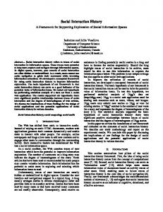
There are several different interventions that may be applied to different groups at different times: vaccination of adults, children and critical workers (V), school closure (S), quarantine of critical workers (Q), and self-isolation (I). The vaccine is assumed to be low efficacy, meaning that only 30% of the individuals vaccinated will be protected. This is representative of a vaccine for a newly emerging strain of influenza. When schools are closed, an adult caregiver is required to remain home with any children under 13 years of age. Sixty percent of the school-children are considered to be compliant, meaning that they remain at home for their entire day. The other 40% participate in their normal after-school activities. Critical workers will be isolated in some type of group quarters in small groups of 16, where they do not come in contact with people outside of their subgroup. When an individual chooses to self-isolate, they withdraw to home and do not participate in any activities away from home. They still contact other people in their household during the times they are at home together. Table 1 describes the four sets of interventions and Figure 4 shows part of the scenario definition. The intra-host disease progression passes through several stages (Committee on Modeling Community Containment for Pandemic Influenza and Institute of Medicine 2006, Halloran et al. 2008). When a person is exposed to the disease, it starts off in a latent stage, where the individual is neither infectious or symptomatic, potentially followed by an incubating stage during which the individual is partially infectious and still does not exhibit symptoms. In the final stage of the disease an individual is fully infectious and display one of four levels of symptoms from asymptomatic to fully symptomatic. The probability of a person staying home instead of participating in their normal activities increases with the severity of their symptoms. Once the disease has run its course, the infected individual is considered recovered and can not be reinfected. Vaccination takes effect at the start of the simulation, the other interventions are triggered when a certain percentage of a subpopulation is diagnosed with the virus. It is assumed that 60% of those who are symptomatic will be diagnosed. School closure is done on a county by county basis, based on the number of sick children who reside in each county. Each person who enters one of the symptomX states has a probability of withdrawing to home, depending on the severity of the symptoms (symptom1 – 20%, symptom2 – 50%, symptom3 – 95%). Sixteen scenarios were simulated, specifying all combinations of the four sets of interventions (I, Q, S, V). Figure 5 shows the number of individuals that are infected for each cell. They can be grouped into four categories: those without vaccination or school closure (labeled a in the figure), vaccination (labeled b), school closure (labeled c), and both vaccinations and school closure (labeled d). Self isolation and quarantine of critical workers have little impact on the overall infection rates. Self isolation happens late into the epidemic (2.5% of the adult population is infected on a single day), limiting its effectiveness. In fact, when school closure or vaccination is included, the trigger level is never reached. Quarantine of critical workers effects such a small portion of the total population (about a third of a percent) that its effects are not apparent in the total population. However, quarantine reduces the percentage of critical workers who are infected from 40% without quarantine to 18% when critical workers are both quarantined and vaccinated, which may be vitally important for maintaining a functioning society. Another interesting phenomenon happens with school closure. Schools are closed when 1% of school children are diagnosed as ill on a particular day in a county. The schools are reopened, on a county by county basis, when the number of diagnosed children falls below 0.1%. Even at that low level, there is enough residual infection to cause another wave of infections. This can be observed in the dual peaks of the group of epicurves labeled b in Figure 5.
2028
Bisset, Feng, Marathe, and Yardi 250000
I Q QI S SI b SQ SQI V VI c VQ VQI VS d VSI VSQ VSQI
Currently infected individuals
a 200000 150000 100000 50000
I Q S V
— — — —
Self isolation Quarantine School Closure Vaccination
0 0
20
40
60
80
100
120
140
160
180
Simulation Day
Figure 5: Currently infected individuals by day for all combinations of interventions. The interventions can be divided into four groups based on the shape of the epidemic curves. Both school closure (b) and vaccination (c) are a significant improvement over doing neither (a), with school closure having the additional benefit of delaying the peak by about a month. Combining school closure and vaccination (d) leads to further improvement.
Number Infected Execution Time
Computation Communication Total
80
1.4e+06
70
1.2e+06
60
1e+06
50
800000
40
600000
30
400000
20
200000
10
100
10
1
0
100
I Q QI S SI SQ SQI V VI VQ VQI VS VSI VSQ VSQI
0
1000
90
Elapsed Time (min)
Number infected
1.6e+06
Execution Time (min)
1.8e+06
Number of PEs
Figure 6: Comparison of execution time and effectiveness for various combinations of interventions. In general, the execution time increases as the complexity of the interventions increases.
Figure 7: Scaling of EpiSimdemics on a California social network containing 33 million individuals. Good performance is seen until 300 cores are used.
Figure 6 shows how the implementation of various public policies effect the execution time of EpiSimdemics. All runs were performed on a 112 node Linux cluster with two 2.2 GHz dual-core Xeon processors and 4 GB of main memory per node. For these runs, 20 nodes (80 cores) were used per cell. There is an increase in execution time of almost 50% between no interventions implemented, and all four implementations implemented. This shows the delicate balance of efficiently implementing public policy and behavior, and allowing modelers to easily specify new policies and behaviors. A specific scenario could be implemented more efficiently, at the cost of making the construction of a new scenario more difficult. As an example of the scaling capability of EpiSimdemics, a network of the state of California, with 33 million people, 5.5 million locations, and 181 million activities, was run with a varying number of processors. The results of these runs are shown in Figure 7. Good scaling is achieved until about 300 cores are utilized. At this point there is simply not enough computation to be done on each core to overcome the communication overhead. EpiSimdemics has been run on social contact networks with over 100 million individuals, and we believe the current system will allow us to simulate the entire US within the next two months.
2029
Bisset, Feng, Marathe, and Yardi 6
SUMMARY AND FUTURE WORK
We have presented EpiSimdemics, a large scale, highly detailed, interaction-based epidemic simulation. It provides a flexible way to specify behavior and interventions in a way that is easy for domain experts to understand and specify, while remaining computationally efficient. We have outlined how this problem can be cast into the framework of succinctly represented partially observable Markov decision process when the underlying state space is described using co-evolving graphical discrete dynamical systems. EpiSimdemics has been used in several sponsor defined case studies, demonstrating real-world applicability. Current work is focused on expanding the scope of EpiSimdemics beyond computational epidemiology, allowing it to be used for a general class of information diffusion processes. Examples of problems that are in this class include the spread of norms and fads through social networks, viral marketing, and the spread of viruses through computer networks. ACKNOWLEDGMENTS We thank the members of the Network Dynamics and Simulation Science Laboratory (NDSSL) and our colleagues at Los Alamos National Laboratory for their collaborations, useful discussions and comments. The work reported here is based on joint effort by current and past members of the NDSSL team. This work is partially supported by NSF Nets Award CNS0626964, NSF Award CNS-0845700, NSF HSD Award SES-0729441, CDC Center of Excellence in Public Health Informatics Award 2506055-01, NIH-NIGMS MIDAS project 5 U01 GM070694-05, DTRA CNIMS Grant HDTRA1-07-C-0113 and NSF NETS CNS-0831633. REFERENCES Anderson, R. M., and R. M. May. 1979, August. Population biology of infectious diseases: Part I. Nature 280:361–367. Atkins, K., C. Barrett, R. Beckman, K. Bisset, J. Chen, S. Eubank, A. Kumar, B. Lewis, A. Marathe, M. Marathe, H. Mortveit, and P. Stretz. 2006. DTRA National Guard study capability demonstration. Technical Report 06-060, NDSSL. Atkins, K., C. Barrett, R. Beckman, K. Bisset, J. Chen, S. Eubank, B. L. A. Marathe, M. Marathe, H. Mortveit, P. Stretz, and A. Vullikanti. 2006. Simulated pandemic influenza outbreaks in Chicago: NIH DHHS study final report. Technical Report 06-023, NDSSL. Atkins, K., C. Barrett, R. Beckman, K. Bisset, J. Chen, S. Eubank, B. L. A. Marathe, M. Marathe, H. Mortveit, P. Stretz, and A. Vullikanti. 2007. An analysis of public health interventions at military bases during a pandemic influenza event. Technical Report 07-019, NDSSL. Barrett, C., R. Beckman, K. Berkbigler, K. Bisset, B. Bush, K. Campbell, S. Eubank, K. Henson, J. Hurford, D. Kubicek, M. Marathe, P. Romero, J. Smith, L. Smith, P. Speckman, P. Stretz, G. Thayer, E. Eeckhout, and M. Williams. 2001. TRANSIMS: Transportation Analysis Simulation System. Technical Report LA-UR-00-1725, LANL. Barrett, C., K. Bisset, S. Eubank, M. Marathe, V. Kumar, and H. Mortveit. 2007. Modeling and simulation of large biological, information and socio-technical systems: An interaction-based approach. In Proceedings of Symposia in Applied Mathematics, Volume 64, 101. Springer. Barrett, C. L., R. J. Beckman, M. Khan, V. A. Kumar, M. V. Marathe, P. E. Stretz, T. Dutta, and B. Lewis. 2009, December. Generation and analysis of large synthetic social contact networks. In Proceedings of the 2009 Winter Simulation Conference, ed. M. D. Rossetti, R. R. Hill, B. Johansson, A. Dunkin, and R. G. Ingalls. Piscataway, New Jersey: Institute of Electrical and Electronics Engineers, Inc. Barrett, C. L., K. R. Bisset, S. Eubank, X. Feng, and M. V. Marathe. 2008. Episimdemics: An efficient algorithm for simulating the spread of infectious disease over large realistic social networks. In Proceedings of the ACM/IEEE Conference on High Performance Computing (SC), 37. IEEE Press. Barrett, C. L., S. Eubank, and M. V. Marathe. 2008. An interaction based approach to computational epidemics. In AAAI’ 08: Proceedings of the Annual Conference of AAAI. Chicago USA: AAAI Press. Beckman, R. J., K. A. Baggerly, and M. D. McKay. 1996. Creating synthetic baseline populations. Transportation Research Part A: Policy and Practice 30 (6): 415–429. Bisset, K., J. Chen, X. Feng, A. Vullikanti, and M. Marathe. 2009, June. EpiFast: A fast algorithm for large scale realistic epidemic simulations on distributed memory systems. In Proceedings of 23rd ACM International Conference on Supercomputing (ICS’09). ACM Press. NYC, NY. Carley, K. M., D. B. Fridsma, E. Casman, A. Yahja, N. Altman, L.-C. Chen, B. Kaminsky, and D. Nave. 2006. Biowar: Scalable agent-based model of bioattacks. IEEE Transactions on Systems, Man, and Cybernetics, Part A 36 (2): 252–265.
2030
Bisset, Feng, Marathe, and Yardi Channakeshava, K., D. Chafekar, K. Bisset, A. Vullikanti, and M. Marathe. 2009, March. EpiNet: A simulation framework to study the spread of malware in wireless networks. In SIMUTools09. ICST Press. Rome, Italy. Committee on Modeling Community Containment for Pandemic Influenza and Institute of Medicine 2006. Modeling community containment for pandemic influenza: A letter report. Washington D.C.: The National Academies Press. Epstein, J. M., J. Parker, D. Cummings, and R. A. Hammond. 2007. Coupled Contagion Dynamics of Fear and Disease: Mathematical and Computational Explorations. SSRN eLibrary. Eubank, S. 2002. Scalable, efficient epidemiological simulation. In SAC ’02: Proceedings of the 2002 ACM Symposium on Applied Computing, 139–145. New York, NY, USA: ACM. Eubank, S., H. Guclu, Anil, M. V. Marathe, A. Srinivasan, Z. Toroczkai, and N. Wang. 2004, May. Modelling disease outbreaks in realistic urban social networks. Nature 429 (6988): 180–184. Ferguson, N. M., M. J. Keeling, W. J. Edmunds, R. Gant, B. T. Grenfell, R. M. Amderson, and S. Leach. 2003. Planning for smallpox outbreaks. Nature 425 (6959): 681–685. Halloran, M. E., N. M. Ferguson, S. Eubank, I. M. Longini, D. A. T. Cummings, B. Lewis, S. Xu, C. Fraser, A. Vullikanti, T. C. Germann, D. Wagener, R. Beckman, K. Kadau, C. Barrett, C. A. Macken, D. S. Burke, and P. Cooley. 2008, March. Modeling targeted layered containment of an influenza pandemic in the united states. Proceedings of the National Academy of Sciences 105 (12): 4639–4644. Kermack, W. O., and A. G. McKendrick. 1927. A contribution to the mathematical theory of epidemics. Proc. R. Soc. Lond. A 115:700–721. Longini, I. M., A. Nizam, S. Xu, K. Ungchusak, W. Hanshaoworakul, D. A. Cummings, and E. M. Halloran. 2005, August. Containing pandemic influenza at the source. Science 309 (5737): 1083–1087. Mundhenk, M., J. Goldsmith, C. Lusena, and E. Allender. 2000, July. Complexity of finite-horizon markov decision process problems. JACM 47 (4): 681–720. National Institutes of Health 2009. http://www.nigms.nih.gov/Initiatives/MIDAS/. NDSSL 2007. Synthetic data products for societal infrastructures and proto-populations: Data set 2.0. Technical Report NDSSL-TR-07-003, NDSSL, Virginia Polytechnic Institute and State University, Blacksburg, VA, 24061. Parker, J. 2007. A flexible, large-scale, distributed agent based epidemic model. In Proceedings of the 39th conference on Winter simulation, 1543–1547. IEEE Press Piscataway, NJ, USA. Smith, R. D. 2006. Responding to global infectious disease outbreaks: Lessons from SARS on the role of risk perception, communication and management. Social Science & Medicine 63 (12): 3113 – 3123. Stewart, W. F., J. A. Ricci, E. Chee, and D. Morganstein. 2003, December. Lost productive work time costs from health conditions in the united states: Results from the American Productivity Audit. Journal of Occupational and Environmental Medicine 45 (12): 1234–1246. AUTHOR BIOGRAPHIES KEITH R. BISSET is senior research associate in the Network Dynamics and Simulation Science Laboratory at Virginia Tech. He received his PhD degree in Computer Science from New Mexico State University. His research interests include high performance computing, parallel and distributed simulation, and modeling complex networks. He is a member of the IEEE Computer Society and ACM. His email address is . XIZHOU FENG is senior research associate in the Network Dynamics and Simulation Science Laboratory at Virginia Tech. He received his PhD degree in Computer Science and Engineering from The University of South Carolina. His research interests include high performance computing, computational biology, bioinformatics, and modeling and analysis of complex systems. He is a member of the IEEE Computer Society and ACM. His email address is . MADHAV M. MARATHE is a Professor of Computer Science, and Deputy Director of Network Dynamics and Simulation Science Laboratory at Virginia Tech. He received his Ph.D. in 1994 in Computer Science from the State University at Albany-SUNY. His email address is . SHRIRANG YARDI is a PhD candidate in the Electrical and Computer Engineering department at Virginia Tech. His research interests include high-performance, power-aware computer architecture, power/performance modeling and optimization, and characterization of new emerging workloads for high-performance computing. He is a member of the IEEE. His email address is .
2031