Modeling Methods and Conceptual Design ... - Semantic Scholar

Afreen Siddiqi Post-Doctoral Research Associate Department of Aeronautics & Astronautics, Massachusetts Institute of Technology, Cambridge, MA 02139 e-mail: [email protected]

Olivier L. de Weck Associate Professor of Aeronautics & Astronautics and Engineering Systems Engineering Systems Division, Department of Aeronautics & Astronautics, Massachusetts Institute of Technology, Cambridge, MA 02139 e-mail: [email protected]

1

Modeling Methods and Conceptual Design Principles for Reconfigurable Systems Reconfigurable systems can attain different configurations at different times thereby altering their functional abilities. Such systems are particularly suitable for specific classes of applications in which their ability to undergo changes easily can be exploited to fulfill new demands, allow for evolution, and improve survivability. This paper identifies the main factors that drive the need for reconfigurability and proposes methods for modeling reconfigurable systems. A survey of 33 different reconfigurable systems is also presented to provide broader insights and general design guidelines for reconfigurable systems. 关DOI: 10.1115/1.2965598兴

Introduction

A common theme in the requirements for many future systems is that they should be able to respond to changing needs. Reconfigurable systems, i.e., those that can change their configurations, can potentially satisfy changing system requirements. The need for reconfigurability is generally driven by three main factors 共see Fig. 1兲. 共1兲 Multiability: the system performs multiple distinctly different functions at different times 共2兲 Evolvability: the system changes easily over time by removing, substituting, and adding new elements and functions 共3兲 Survivability: the system remains functional, possibly in a degraded state, despite a few failures These three situations either uniquely or in a combination envelope almost all cases for which reconfigurability may be desired. The requirement for multiability can be due to the resource efficiency considerations or for performance enhancement. In both cases, the essential requirement on the system is that it needs to fulfill multiple objectives/goals, and thus should be capable of executing them collectively, but not necessarily simultaneously. Reconfigurability in systems is also often an enabler of change over time. The future configurations may be known a priori at the time of design or they may be unpredictable in which case the evolvability helps to manage uncertainty. Reconfigurability can also be a means for enhancing a system’s survivability. In the event of partial failure, reconfigurable systems can potentially configure to a state in which some level of functionality is maintained. Furthermore, they can enhance the safety margins 共through reconfigurations兲, and thus effectively reduce the probability of experiencing failure. The life cycle of a reconfigurable system can be partitioned into phases, as shown in Fig. 2. The reconfiguration phase in which the system undergoes changes in its configuration 共after it has been fielded兲 sets these systems apart from the traditional nonreconfigurable ones. Therefore, new frameworks that account for the time related changeability aspects of reconfigurable systems can be useful for analysis and design for reconfigurability. 1.1

Literature Review. From a review of current literature, it

Contributed by Design Theory and Methodology Committee of ASME for publication in the JOURNAL OF MECHANICAL DESIGN. Manuscript received April 26, 2007; final manuscript received March 4, 2008; published online September 10, 2008. Review conducted by Yan Jin.

Journal of Mechanical Design

becomes clear that there has been an increasing effort toward the study and design of systems that can change or reconfigure. Figure 3 shows how the number of journal articles on this topic has increased over the past few years. The most extensive work related to reconfigurable systems has been done in the computing domain. Field programmable gate arrays 共FPGAs兲, devices that allow circuits to be defined in software and provide for easy reconfigurations, have advanced greatly in recent years 关2兴. Avionics systems that can evolve with changing environmental conditions of a spacecraft have been developed to enhance survivability in long duration space missions 关3兴. Various concepts of softwareradio based transponders for communication satellites have been proposed that allow for on-orbit reconfigurations 关4,5兴. Manufacturing systems have also received significant attention for reconfigurability. The National Research Council has identified reconfigurable manufacturing systems 共RMS兲 as the number one priority technology for future manufacturing in 2000 关6兴. Several researchers have especially focused on developing design methods for reconfigurable machine tools 共RMT兲. The general scheme is that from a set of commercially available modules 共that constitute a module library兲 the optimal RMT design is formulated so that it has the desired reconfigurability in its degrees of freedom, work piece geometry variability, spindle orientation, etc. 关7兴. Reconfigurability has also been increasingly incorporated in the design of new air and space systems. Unmanned aerial vehicles 共UAVs兲 that can morph their wings in-flight in order to efficiently carry out different roles have been the subject of much recent research and development 关8,9兴. These UAVs can undergo large changes in wingspan, area, and sweep angles so that the same vehicle is able to effectively perform loiter/reconnaissance and attack roles in a single mission. For reconfigurable spacecrafts, two kinds of approaches have been mainly explored. The first involves a “plug and play” architectural approach in which spacecrafts are built from a standard set of modules that supposedly allow for faster manufacturing and potentially on-orbit reconfigurations/upgrades, etc. 关10兴. The second approach involves modular architectures based on common elements of form such as truncated octahedrons 关11兴 and tetrahedrons 关12兴, etc. Several research efforts have also focused on developing frameworks and methodologies for designing changeable 共sometimes also referred to in literature as flexible or adaptable兲 systems. Some examples include a framework that has been developed for multiattribute decision making in flexible system design 关13兴, transformer design theory 关14兴 that deals with form related aspects of systems capable of configuring into different states, and selection integrated optimization methodology 关15兴 that can be used to study adaptability in design variables. It is important to recognize that analysis methods specifically

Copyright © 2008 by ASME

OCTOBER 2008, Vol. 130 / 101102-1

Downloaded 24 Mar 2009 to 18.111.23.51. Redistribution subject to ASME license or copyright; see http://www.asme.org/terms/Terms_Use.cfm

Fig. 1 Properties enabled by reconfigurability

catering to the key characteristics of reconfigurable systems 共i.e., their time varying nature兲 can be especially effective for producing good designs. In this regard, a few modeling methods for analyzing reconfigurable systems are presented. These methods can be used for a wide variety of systems, and their applicability is illustrated through examples of a planetary rover and a morphing aircraft. The modeling techniques are then followed by a review of the physical design of several different kinds of reconfigurable systems. Based on this review, some guidelines are formulated that can help in the development of good design concepts for reconfigurable systems. 1.2 Reconfigurable Systems: Definition. Reconfigurable systems can be defined as those systems that can reversibly achieve distinct configurations 共or states兲, through alteration of system form or function, in order to achieve a desired outcome within acceptable reconfiguration time and cost. Reconfigurable

systems in this discussion are thus limited to those that do not go through only a one-time change. Rather they are capable of changing states repeatedly in the operational stage of their life cycle. The set of configurations S of a system is taken to be the 共usually finite兲 collection of specific discrete or continuous states of the system, in which there is a different form and/or functional behavior. Figure 4共a兲 shows an object-process diagram 共OPD兲关16兴 of a reconfigurable system, as defined above. It is shown that in a reconfigurable system the attributes of the system form, the externally delivered function, and/or the attributes of the function are affected by the process of reconfiguration. For example, consider a recently developed morphing UAV, the MXF-1, which can reversibly reconfigure its wings during flight. It can achieve an infight area change of 40%, a span change of 30%, and a wing

Fig. 2 Stages in life cycle of a reconfigurable system

Fig. 3 Number of journal articles published with the keyword “reconfig” in the title or abstract „Ref. †1‡…

101102-2 / Vol. 130, OCTOBER 2008

Transactions of the ASME


(a)

(b)

Fig. 4 Object-process diagrams of reconfigurable systems: „a… OPD of a reconfigurable system; „b… OPD of a morphing UAV

sweep variation of 15– 35 deg 关9兴. An OPD of such a vehicle is shown in Fig. 4共b兲. The MXF-1 wing has an articulating lattice structure. Its skin is of a material that can undergo strains in excess of 100% and conforms to the wing’s changing skeleton. The geometry change is achieved through a series of internal linear electromechanical actuators. The reconfigurable wings optimize the aircraft for dramatically different flight conditions—for instance, from an efficient, high-altitude loiter shape to an efficient high-speed attack mode 关9兴. Figure 5 shows a subscale prototype of this UAV.

2

Modeling Reconfigurable Systems

Since reconfigurable systems can attain different configurations over time, the modeling methods used for their analysis should account for their time varying nature. It is proposed that Markov models and control-theoretic approaches can be used to model such systems effectively. These approaches are developed in this section, and their applicability for analyzing dynamical aspects of reconfigurable systems is demonstrated through a few examples. 2.1 Markov Models. A Markov process is a probabilistic model of usually a complex system, which employs the concepts of states and state transitions. Reconfigurable systems can therefore be studied with Markov models in a very natural way. The Markov theory has been fairly well developed since its first introduction by the Russian mathematician A. Markov in 1907 关18兴. 2.1.1 Discrete-Time Markov Chains. A discrete-time Markov chain is a process in which the system’s state changes at certain discrete-time instants. Suppose a system can exist in N finite and discrete states that belong to a set S = 兵1 , 2 , . . . , N其. A time ordered set, T = 关t1 , . . . , tn , . . . , t f 兴 can be defined, and the system state at a time instant tn can be denoted as Xn. Then, for a Markov process the following assumption holds 关19兴:

pij共n兲 = Pr兵Xn+1 = j兩Xn = i其,

i, j 苸 S

共1兲

where pij共n兲 is the probability of transitioning from States i to j at time tn. The probability law of the next state Xn+1 depends on the past only through the present value of the State Xn. In other words, the Markovian property refers to a condition where the memory of previously visited states between t1 , . . . , tn−1 is irrelevant. The pij共n兲 are also called the single-step transition probabilities since they define the transition probabilities for one-time step only. The transition probabilities from a State i sum to 1. Using the transition probabilities between each state pair, the complete system can be described by defining a single-step transition probability matrix P共n兲:

P共n兲 =

冤

p11 ¯ p1N ]

]

]

pN1 ¯ pNN

冥

共2兲

This matrix provides full information regarding the behavior of the system at a particular time instant. In order to determine the individual state probabilities, a vector ␲共n兲 is defined where ␲共n兲 = 关␲i共n兲兴1⫻N, and ␲i共n兲 is the probability of being in State i at time tn. The state probabilities at time tn+1 are then simply

␲共n + 1兲 = ␲共n兲P共n兲

共3兲

If the initial state of the system is known 共i.e., ␲共0兲 is given兲, then the above relationship allows the state probabilities to be calculated at any tn. At any time instant, the state probabilities need to sum to 1, i.e., N

兺 ␲ 共n兲 = 1 i

共4兲

i=1

The case in which the single-step state transition probabilities do not depend on time is known as the time-homogeneous Markov chain. For systems whose state probabilities reach a limiting value as n gets larger 共which is when the system is not periodic and is homogeneous兲, the asymptotic or steady-state behavior of ␲ is 关18兴

␲共⬁兲 = lim ␲共0兲Pn n→⬁

共5兲

Since at steady state, the relation ␲ = ␲ P has to hold true: ␲共⬁兲 can be computed by solving the simultaneous equations given by N

␲ j共⬁兲 = Fig. 5 NextGen MXF-1 morphing UAV †17‡


兺 ␲ 共⬁兲p , i

ij

j = 1,2, . . . ,N

共6兲

i=1

OCTOBER 2008, Vol. 130 / 101102-3


(a)

Fig. 7

Fig. 6 Markov model of a generic reconfigurable system

(b)

Markov model of operational and reconfiguration states

while pi-ij is the transition probability from i to State ij. With this notation 共and omitting the argument 共⬁兲 for the ␲s for simplicity兲, for the type of systems shown in Figs. 6 and 7, the results given in Eq. 共6兲 lead to the following equations for steady-state behavior: k

␲i = pi−i␲i +

Since these N equations are linearly dependent, in order to get a nontrivial solution, only N − 1 equations are used, and the Nth equation is the property that all state probabilities should sum to 1. i

共8兲

兺␲ p

ji ji−i

␲i =

i=1

101102-4 / Vol. 130, OCTOBER 2008

j⫽i

k

共7兲

It can be seen that the homogeneous Markov chains are quite amenable for analysis since the state probabilities can be predicted for any future time given an initial state. This allows calculation of useful statistics such as average time spent in a particular state, mean time before a certain state may be reached for the first time, and so on 关19兴. In the case of reconfigurable systems, the homogeneous model is applicable if the single-step transition probabilities are the same over the system’s operational time. A general model of a reconfigurable system can be constructed, as shown in Fig. 6. Two types of states are shown: operational states and reconfiguration states. Operational states are those in which the system operates and carries out its useful function. In the figure, they are States A and B 共that are shaded兲. The reconfiguration states are those in which the reconfiguration processes are carried out, and the system may be 共but not necessarily兲 fully or partially disabled. For the most general case, it can be assumed that each operational state can configure into every other operational state after passing through a specific reconfiguration state. Thus, State A can transition to State AB 共which is a reconfiguration state in which the system reconfigures from A to B兲, and then State AB goes on to State B 共which is the state in which the system is in operational configuration B兲. A similar path is shown for B to BA to A. The self-transition probabilities pAB-AB and pBA-BA in the reconfiguration states can be used to account for factors such as reconfiguration delay or failure in any particular reconfiguration attempt. In essence, they capture the expected delay in moving from one operational state to the next. In most real systems, it is usually not possible to enter each operational state from every other operational state. However, the most general case is considered here for completeness. For the type of system shown in Fig. 6, for k operational states, there are k共k − 1兲 reconfiguration states. In the general case, Fig. 7 shows a generic operational state and a reconfiguration state. In order to clearly differentiate between the types of states, each operational state is denoted by a single variable i or j, etc. The reconfiguration states are denoted by two variables, so, for instance, ij is a reconfiguration state that converts State i to State j. A hyphen in the subscript of the transition probabilities serves to indicate the initial and final states between which the transition takes place. Thus, pi-i is the self-transition probability of State i,

ji ji−i,

j=1

N

兺 ␲ 共⬁兲 = 1

兺␲ p

j=1

j⫽i

,

1 − pi−i

共9兲

where

␲ ji =

p j−ji ␲j 1 − p ji−ji

共10兲

Combining the above two relations gives k

␲i =

兺

1 p j−ji p ji−i ␲ j, 1 − pi−i j=1 1 − p ji−ji

j⫽i

共11兲

Since the transitions to reconfiguration states have the specific form, as shown in Fig. 7, it is also true that 共12兲

p ji−ji + p ji−i = 1 Using this result, Eq. 共11兲 becomes k

␲i =

兺

1 p j−ji␲ j, 1 − pi−i j=1

j⫽i

共13兲

To obtain a nontrivial solution, Eq. 共7兲 is also used. In order to have a relation only in terms of the operational states, Eq. 共7兲 can be written by explicitly separating out the operational 共␲ j兲 and the reconfiguration state 共␲ij兲 expressions: k

k

k

兺␲ +兺兺␲ j

ij

= 1,

i⫽j

共14兲

i=1 j=1

j=1

Using Eq. 共10兲, it becomes k

k

k

兺␲ +兺兺 1−p

p j−ji

j

j=1

i=1 j=1

␲ j = 1,

i⫽j

共15兲

ji−ji

Thus, the asymptotic k operational state probabilities can be determined directly using the k − 1 linear equations given by Eq. 共13兲 and the kth equation given by Eq. 共15兲. Note that it is assumed that the self-transition probabilities pi−i and p ji−ji are not 1. A simple example of a planetary rover can now be used for illustrative purposes. It is considered that the rover has three distinct configurations during its operation. Suppose the three configurations, or states, correspond to its operation on flat terrain 共which mainly involves driving activities and is denoted as State D兲, its ascent or descent of a crater slope 共which is denoted as C to indicate climbing up or down兲, and its exploration of a crater Transactions of the ASME


Fig. 8 Markov model of reconfigurable rover

floor 共mainly carrying out scientific investigations and is denoted as S兲, respectively. The reconfigurable rover can employ wheels or legs for its locomotion. Therefore, it is conceivable that the wheels are used in the flat terrain driving configuration, while the legged configuration is used when climbing/descending slopes, etc. Suppose the terrain in which the rover will operate is fairly well known. Its characteristics 共based on crater density, etc.兲 are such that a Markov model, shown in Fig. 8, can be constructed. This is only a notional case, and the assumption is that a typical mission can perhaps be described in this way given relevant parameters such as terrain profile, robot speed, mission duration, reconfiguration processes, and chances of irrecoverable failure in each state, etc. The evolution of the operational state probabilities, ␲i for i = 1 , 3 , 5, for a number of time steps is shown in Fig. 9. Each iteration can represent a certain period of time 共days, weeks, etc.兲 Using Eqs. 共13兲 and 共15兲 the steady state analytic results are found to be ␲1 = 22.32%, ␲3 = 17.08%, and ␲5 = 24.8%. This is in agreement with the results shown in the plots of Fig. 9, which were

computed numerically. In many cases, it is often desirable or even required to model the failure aspects of the system as well. In such a situation, a model can be employed in which a failed state F, from which the system cannot recover, is also factored in. This type of model would essentially describe a system in which the failed state is an absorbing state from which once the system enters it can never leave. There are analytical means of determining the expected number of iterations after which a system will enter an absorbing state, and those can be employed to determine failure time, etc. 关19兴. For the rover example, Fig. 10 shows a Markov model in which a failed state has been included. Various insights can be gained about the system’s behavior through such a model. For instance, Fig. 11 shows the chances of being in any operational state 共i.e., po = ␲D + ␲C + ␲S兲 and the chances of being in any reconfiguration state 共which is pr, and is the sum of all the probabilities of reconfiguration states兲. Since the failure probability is very low initially, the pr is almost equal to 1 − po. It can thus be determined how likely it is for the system to be performing useful work, 共i.e., it exists in an operational state兲. This type of analysis can help in evaluating the effectiveness of the design. With these models one can also determine the effects of changing probabilities of self-transition of reconfiguration states. These essentially capture characteristics of the reconfiguration process and can be used in making specific design choices. Figure 12 shows how the total probability of being in any operational state D, C, or S 共i.e., ␲D + ␲C + ␲S兲 is affected when the self-transition probabilities pDC−DC, pCD−CD, pSC−SC, pCS−CS, pDS−DS, and pSD−SD are reduced by 10% from the values shown in Fig. 10. Thus, by varying these self-transition probabilities, which correspond to design issues of the reconfiguration processes, the effect on the system performance can be determined. The example of a reconfigurable UAV 共described in the previous section兲 can also be used to further illustrate the application of this method. Figure 13 shows a Markov model that describes the states of the UAV along with the notional transition probabilities 共which in reality would be based on military strategic scenarios, likelihood of finding attack targets in an area, etc.兲 It is assumed that the vehicle can exist in two operational states—a swept low aspect ratio wing configuration for dash 共D兲 and an unswept high

Fig. 9 Rover operational state probabilities


OCTOBER 2008, Vol. 130 / 101102-5


Fig. 10 Markov model of reconfigurable rover with a failure state

aspect ratio wing configuration for loiter 共L兲. The aircraft also has reconfiguration states that correspond to the two operational states along with a nonrecoverable failure state 共F兲. The evolution of state probabilities in this case was computed for 400 steps, and the first 80 iterations are shown in Fig. 14. Figure 15 shows the probability of the system being in the failed state. Three plots were generated by varying the transition probabilities leading to State F 共such as pD−F, pL−F, etc.兲. In the first line 共from the top兲, the failure probabilities were increased by 20% from the values shown in Fig. 13. In the second plot, the failure probabilities are those shown in Fig. 13, while in the third plot they have been reduced by 20%. With decreasing values of those transition probabilities 共denoted collectively as P f in Fig. 15兲, the chance of being in the failed state decreases. Depending on how much that decrease is, trades can be carried out between reliability and cost 共since it can be expected that there will be increased cost in bringing down the failure probabilities兲. In this simple model, only one irrevocable failed state is considered 共since the primary aspect of interest is the multiability of the

Fig. 11 Operational and reconfiguration state probabilities

101102-6 / Vol. 130, OCTOBER 2008

UAV兲. For a more detailed analysis of survivability considerations, such as of graceful degradation, more states will need to be factored, capturing the degraded behavior/performance. These examples illustrate the use of homogenous Markov models as potential tools for analysis of reconfigurable systems. In many actual applications, determining the appropriate values for transition probabilities can be difficult. Furthermore, the applicability is limited to a class of systems in which no active decision rule is used to determine the state to which the system should reconfigure rather the probabilities are assumed to be known. There are many types of systems in which the reconfiguration to a state will depend on some exogenous variable that will make some states desirable and some undesirable as a function of time. The different kinds of Markov models can be used in such cases and are discussed in the following section. 2.1.2 Time Varying Markov-Based Models. A more general case is the one in which the single-step transition probability matrix P is not the same for every time step. This is known as the

Fig. 12 Effect of 10% change in self-transition probabilities of reconfiguration states



have an associated Ji for the given u共n兲, and the state transition probabilities will be according to this Ji. The optimal state i* will have the highest probability for the system to transition into, followed by the next best state, and so on. The states that are worse than the existing configuration can be modeled to have extremely low transition probability for that time period. For a given input u共n兲, the optimal operational state is i* = arg max J共u,S兲

共18兲

where J is some function that needs to be maximized, and S is the set of system states. Also as described above, pm−mj ⬎ pm−mk, Fig. 13 Markov model of a reconfigurable unmanned aerial vehicle

nonhomogeneous Markov chain 关20兴. In this case, Eq. 共5兲 does not hold, and analytical solutions to the asymptotic behavior of the system are not possible 共except for the periodic cases兲. Indeed the system may not have a steady-state as is possible for the case of homogeneous systems. The multistep transition probabilities are computed by taking a complete product of each P共n兲关18兴: ⌽共m,n兲 = P共m兲P共m + 1兲, . . . ,P共n − 1兲,

mⱕn−1

共16兲

Most reconfigurable systems can be better described through nonhomogeneous models, with a further assumption that the state transition probabilities at each time instant are conditioned on some external time-varying process u共n兲. Thus for any State-Pair i and j 共and using the notation with the hyphen兲 pi−j共n兲 = f共u共n兲,i, j兲

共17兲

This u共n兲 can be mapped to a corresponding behavior of the system such that some objective J is achieved. From a given set of finite states that the system can attain in one step, there will be a state i* that is most desirable for the system to have for a particular u共n兲 and a particular formulation of J. In fact, each state will

J j ⬎ Jk ⬎ Jm

共19兲

where pm−mj is the probability that operational state m will transition to the reconfiguration state mj and so on. Note, that u共n兲 could be a vector, making J共u , S兲 more complex. Also, one of the reasons that pij is probabilistic is due to the estimation error of u共n兲 among other factors. As an example, consider a reconfigurable satellite constellation that is capable of changing its coverage to different locations on the globe in response to disaster relief efforts. For simplicity, it is assumed that it can attain a set of discrete states. The input to this system is the stochastic process of disaster occurrence 共e.g., floods, earthquake, and hurricane兲 in various regions of the globe. Given a certain demand at a particular time u共n兲, there is an optimal state 共among the discrete and finite set兲 that the satellite constellation should adopt so that it maximizes its communication service and coverage to the required region. The Function J can thus be the revenue 共or perhaps some metric of service兲, and the state that maximizes J should get the highest transition probability for that time step. Thus, the transition probabilities will be such that p j−ji* are high 共i.e., the probability of moving from a suboptimal state to its corresponding reconfiguration state that leads to i* will be high兲. Also, if the system is already in the optimal state, it will stay there, i.e., pi*−i* = 1 and pi*−i* j = 0. In other words, it will be an absorbing state but only during the period of time when its optimal. Since in the nonhomogeneous case, the absorbing states change with time 共with the exception of irrevocable failure兲, the long-term behavior

Fig. 14 Evolution of UAVs state probabilities


OCTOBER 2008, Vol. 130 / 101102-7


Fig. 15 Effect of 20% increase and decrease in failure probability over time

cannot be predicted analytically 共unless u共n兲 is periodic兲. One way to assign pijs is to establish a rule that a state transition will occur if the “net benefit” Fij is positive, where Fij = ⌬Jij − Cij

共20兲

⌬Jij = J j − Ji

共21兲

The ⌬Jij essentially is the difference in performance of the two States i and j and should be positive for a transition to occur 共i.e., the system moves toward a better state兲. Additionally, Cij represents the cost of transitioning from i to j. Note that by this definition, remaining in the same state incurs no additional benefit or cost: Fij = 0,

i=j

共22兲

If Fij ⬎ 0 then it means that there is a net benefit to be gained by transitioning from i to j even while accounting for the costs involved. One possible formulation for pij can be pij =

Fij

兺F

,

j 苸 S⬘

共23兲

ij

j

where S⬘ 債 S and consists of states for which Fij ⬎ 0. A detailed discussion and application of this method to reconfigurable planetary rovers is provided in Ref. 关21兴.

2.2 Metacontrol Framework. Another scheme of modeling and representing reconfigurable systems can be based on concepts and tools of classical control theory. Control-theoretic approaches have been used in a metasense for a variety of applications ranging from modeling organizational dynamics to human-machine interaction 关22兴. These are systems that cannot be described through physical dynamical equations; nonetheless the tools of control theory lend themselves to studying certain basic timerelated characteristics of such systems. It is proposed that a control-theoretic approach can also be applied to a class of reconfigurable systems that can undergo two kinds of reconfigurations: online reconfiguration and off-line reconfigurations. In the former case, the system continues its operation as it reconfigures, while in the latter case it is nonoperational during the reconfiguration process. For instance, a rover may undergo online reconfigurations as it explores the surface of a planet, or it may be reconfigured off-line 共by a crew in a manned exploration mission兲. Figure 16 shows how online and off-line reconfigurabilities can be modeled in a generic manner. Typically, there is some change in the system’s environment 共such as planetary surface terrain for a rover or strategic conditions in a military zone兲. Those changes are sensed and mapped to some corresponding desired attribute of the system 共such as the desired characteristics of a rover’s wheel in response to terrain conditions, wing geometry of a UAV in

Fig. 16 Generic reconfigurable system

101102-8 / Vol. 130, OCTOBER 2008



extent of each wing’s in-flight reconfigurability would be determined so that the overall system performance across all the operational scenarios of interest is satisfied to some desired level/ goal. A more detailed discussion on the application of these methods can be found in Ref. 关21兴, where it is shown how the states of a reconfigurable wheel may be determined for application in planetary surface exploration vehicles. It should be noted that these modeling methods have to factor in the available computational resources. The computational requirement may become significant for a real world complex system. In such a case, the issue may be addressed by balancing the time fidelity of the simulations versus the number of modeled states so that the problem is reduced to a computationally manageable size.

Fig. 17 Online and off-line reconfigurations

response to changing mission needs.兲 The reconfigurable system tries to achieve the desired configuration through its online reconfiguration loop 共which is essentially the traditional type of active control in many modern systems兲. If the online reconfiguration bandwidth, i.e., the limits to which the system can configure online, are not sufficient for fulfilling the desired objective, then the system goes through its off-line reconfiguration process. Through off-line reconfiguration, it undergoes changes such that it can achieve the desired states once it is operational again. The set of states or configurations that the system can adopt through off-line reconfiguration can be represented as A = 兵A1,A2, . . . ,An其

共24兲

Each configuration Ai has its specific online reconfiguration range ␦Ai defined as

␦Ai = aimax − aimin

共25兲

This defines the extent to which the system can adapt itself while in operation in a particular state Ai. Through the combination of online and off-line reconfigurabilities, the total range of an attribute that the system can change through reconfiguration is enlarged 共as illustrated through Fig. 17兲. It is possible, however, that this total range/reconfiguration bandwidth may not always be continuous. If the example of a reconfigurable UAV is considered again, one can conceive of a design that can go through both online and off-line reconfigurations. The online reconfiguration would involve in-flight wing geometry changes. The off-line reconfigurations 共performed between sorties of the vehicle兲 can potentially involve switching out components 共perhaps even wing modules兲, payload, etc., such that the most suitable ones are used for different usage scenarios. Note, that, traditionally, what is being referred to as online and off-line reconfigurabilities has been studied separately 关23,24兴. This approach however, by combining the two types of reconfigurations, can allow for exploring a larger design space for the system. The metacontrol framework expands the spectrum of possibilities that can be assessed for the system. The three methods discussed above provide ways to model and assess the time related aspects of reconfigurations. The Markov approach allows for analyzing operational, reconfiguration, and failure states. Figures 12 and 15 show examples of how the effects of changes in self-transition or failure probabilities can be evaluated and then possibly traded in the design process. One can quantify the effect of change in failure probabilities through such analysis and then translate the results into design 共or performance兲 requirements for subsystems. Such requirements in turn guide decisions on selecting components. The analysis of reconfiguration time aspects 共as allowed by the metacontrol framework兲 can lead to a definition of requirements on the physical design such as choice of actuators and mechanisms. Similarly, through the analysis of A 共number of off-line configurations兲 and ␦Ai 共extent of online reconfigurability兲, one can produce requirements for system form. Such as in the case of a reconfigurable UAV, the number of wing types 共that can be fitted on to the aircraft兲 and the Journal of Mechanical Design

3

Survey of Reconfigurable Systems

The preceding sections discussed various theoretical notions— definitions and modeling techniques—for studying reconfigurability. In order to gain broader insights for implementation of reconfigurability, a survey was conducted on a set of different types of reconfigurable systems. This section presents some of the common trends that were observed and guidelines that were elicited from analyzing their designs. 3.1 Systems Description. A set of 33 different systems ranging from a simple potentiometer to a large complex radio telescope system, the very large array 共VLA兲, was selected for the study. Some of their basic information is given in Table 1 and more details are provided in Ref. 关25兴. The Functional Type in Table 1 has been assigned based on the definitions proposed in Ref. 关43兴. The letters E, M, and I represent energy, matter, and information, respectively. The number 1 is associated with functions that transform or process the operand, 2 is for transport or distribute, 3 is for store or house, 4 is for exchange or trade, and 5 is for control or regulate 关43兴. It can be seen that the selected systems mostly are described by M1, M2, M3, and I1 types, i.e., most of these systems are matter or information processing 共M1, I1兲, or mass transportation 共M2兲, or storage/housing 共M3兲. Note that these types are associated with the primary function of the system, for there are certainly several other subprocesses that are of different types and enable the primary function to be carried out. It should be noted that these systems range from conceptual stage 共e.g., variable diameter compound helicopter兲 all the way to full production and deployment stage 共e.g., SMART car兲. Some kind of data such as cost, etc., however, could not be obtained for all the 33 systems, and thus there are some empty cells in Table 1. 3.2 System Requirements. The three system properties that were identified for driving the need for reconfigurability in Sec. 1 were matched against the stated requirements for each systems. In order to get any meaningful insights, the systems were classified in three application categories of commercial/consumer items, air/ space systems, and manufacturing/test systems. Systems 1–15 共i.e., from potentiometers to race car in Table 1兲 were the commercial/consumer items, systems 16–18 共NI-RIO to RMS兲 were manufacturing/test, and systems 19–33 共Polybot to VLA兲 were designated as air/space systems. In this analysis, the multiability property was refined into two subcategories of “resource efficiency” and “multiple configurations” 共see Fig. 1兲. These categories along with the other two 共evolvability and survivability兲 were then assigned to each system based on their stated objectives and requirements as found in their description and other relevant literature sources. A 33⫻ 4 matrix was created in which a value of 1 was assigned to the element in the ith row and jth column if the ith system fulfilled the jth need subcategory. The fraction of systems assigned to each of these four categories 共for each of the three application domains兲 was determined and is shown in a plot in Fig. 18. It can be seen that the different classes show varying trends in OCTOBER 2008, Vol. 130 / 101102-9


Table 1 Set of systems used for reconfigurability analysis. Legend: E, energy; M, mass; I, information; 1, transform; 2, transport or distribute; 3, store or house; 4, exchange or trade; 5, control or regulate No.

Name

1 2 3 4 5 6 7 8 9 10 11 12 13 14 15 16 17 18 19 20 21 22 23 24 25 26 27 28 29 30 31 32 33

Potentiometer Airpot 共adjustable shock absorber兲关26兴 LEGO Vaccum Food processor Sewing machine Convertible stroller 关25兴 Digital photoframe USM Haller table 关27兴 3-in-1 crib Sofa bed Adjustable bed Convertible car SMART car 关28兴 Flexible race car 关23兴 Reconfigurable input/output 共NI-RIO兲 device 关29兴 Reconfigurable discrete die 关30兴 RMS 关6兴 Polybot 共reconfigurable modular robot兲关31兴 LARA 共reconfigurable rover兲关32兴 SRR 共sample return rover兲关33兴 Solar maximum mission 共SMM兲关34兴 SWARM 共reconfigurable spacecraft兲关35兴 Xilinx Virtex II Pro FPGA Evolvable hardware 共EHW兲关3兴 Long life spacecraft avionics 关36兴 Reconfigurable communications equipment 共RCE兲关37兴 Reconfigurable patch antenna 关38兴 TTC transponder 关5兴 MXF-1 共Morphing UAV兲关9,39兴 F-14 Tomcat 关40兴 Variable diameter compound helicopter 共VDCH兲关41兴 Very large array 共VLA兲关42兴

the reasons for their reconfigurability. The consumer items are dominated by the two subcategories of multiability. They either are reconfigurable due to resource efficiency requirements or have multiple-configurations for some planned or unplanned usage needs. Space systems, on the other hand, are motivated by requirements of survivability and evolution for unknown configura-

Fig. 18 Reconfigurability drivers for systems in three application domains

101102-10 / Vol. 130, OCTOBER 2008

Functype

Mass 共kg兲

Volume 共m3兲

Cost 共$兲

E1 E1 M1 M4 M1 M1 M2 I3 M3 M3 M3 M3 M2 M2 M2 I1 M1 M1 M2 M2 M2 I1 I2 I1 I1 I1 I1 E4 I1 M2 M2 M2 I4

0.01 0.07 1 7.5 6 9.18 4.09 0.82

1 ⫻ 10−6 7.6⫻ 10−5 3 ⫻ 10−3 6.88⫻ 10−2 1.5⫻ 10−2 4.7⫻ 10−2 2.9⫻ 10−1 8.6⫻ 10−4

36.4 41.8 61.4 1590 730 500 2 3980 32,700 3.6 50 10 2320 25 0.001

1.44 2.74 1.02 12 5.63 7.99 9.35⫻ 10−4 2 166 2.3⫻ 10−3

2.5 20 14 650 150 130 70 200 5000 250 550 2700 35,000 14,000 99,500 2000 500,000 1 ⫻ 106 10,000

16 2.9 45.45 33,800 9550 6.2⫻ 106

6.36 3.16⫻ 10−2 7.29⫻ 10−6 6.25⫻ 10−6 4.05⫻ 10−3 1.82⫻ 10−4 1.25⫻ 10−6 6.97⫻ 10−3

1.2⫻ 108

1820 90.6 376,000

3.8⫻ 107 1 ⫻ 108 7.9⫻ 107

250 180 500 80

tions in addition to multiability. In manufacturing, the system resource efficiency, the multiple-configurations, and the evolution aspects all play a key role. 3.3 Reconfiguration Time. The time related aspects were studied for the systems for which relevant data could be obtained. The reconfiguration time, denoted as Tr, is the time a system takes to reconfigure from one state or configuration to its next state/ configuration 共see Fig. 6兲. Depending on the context it may include the total time spent in determining the new configuration 共e.g., in case of evolution兲 in addition to the actual time spent in carrying out the reconfiguration processes on/by the system. The surveyed systems for which reconfiguration time information could be obtained are listed with relevant data in Table 2. For consumer items such as vacuum cleaners and food processors, the time was estimated from personal experience as a user of these systems, whereas for other systems such as the F-14, and VLA, the reconfiguration time was obtained from actual data. In the case of the solar maximum mission 共SMM兲, the reconfiguration time was taken to be the total time it took for servicing the craft 共which was 2 days, since the first attempt to capture the satellite failed on the first day of the mission兲关34兴. It does not include the time of getting the mission approved, ready, and launched to carry out the reconfiguration. In the case of SWARM also, the time is the docking time for the various modules based on the assumption that the docking-undocking procedures are what primarily constitute the reconfiguration process in the SWARM system 关25兴. For NI-RIO the data are again based on Transactions of the ASME


Table 2 Reconfiguration times No.

Name

4 5 6 7 8 10 11 12 13 14 16 17 19 22 23 30 31 33

Vaccum Food processor Sewing machine Convertible stroller Digital photoframe 3-in-1 crib Sofa bed Adjustable bed Convertible car SMART car NI-RIO Reconfigurable discrete die Polybot SMM SWARM Morphing UAV F-14 Tomcat VLA

Reconfiguration time

Average state occupancy time

Life 共yr兲

30 s 60 s 10 s 3 min 5 min 30 min 5 min 60 s 3 min 2 days 15 min 30 min 30 s 2 days 120 s 10 s 6s 14 days

15 min 20 min 3 min 30 min 1 day 12 months 8h 2h 30 min 3 months 8h 20 h 5 min 5 yr 30 min 5 min 15 min 3 months

2+ 2+ 2+ 1+ 3+ 2+ 5+ 2+

personal experiences as a user, and for the reconfigurable discrete die, the data are based on a first order estimate and are meant to only capture the order of magnitude of the time. The average time the system spends in a particular state or configuration, denoted as Ts, was considered to be the average state occupancy time. For instance, the VLA stays in each of its four configurations A, B, C, and D for three months on average. So the Ts for the VLA is 3 months. For consumer items, and other items such as NI-RIO or the reconfigurable discrete die, the Ts was again estimated from general experience and basic assumptions. The log of the ratio of Ts and Tr was computed and plotted, as shown in Fig. 19. An interesting observation that can be made is that there is a lower bound of approximately 1 for this ratio, i.e., the reconfiguration time is never more than at least 1 / 10 of the time the system spends in a particular configuration. One might state that reconfiguration times that exceed 10% of the useful time in any given state render reconfiguration undesirable. The truly acceptable maximum Tr depends on the exogenous dynamics 共also discussed earlier in Sec. 2兲. Note that this fact distinguishes reconfigurable systems from pure redesign or unplanned remodeling. This 10% rule can perhaps be used as a useful rule of thumb when considering the design of a system that needs to reconfigure between different states. It should be noted that where the data have been estimated from experience or on a first order level, the lower limit for the state occupancy time and an upper limit for the

5 – 7+ 5+ 5+ 30+ 共7200 op h兲 30+

reconfiguration time have been used. Therefore, in reality, on average the state occupancy time for most of these systems will be longer, and the reconfiguration time will be shorter. The ratio will therefore be even higher, and the proposed ratio of at least onetenth should still hold. 3.4 Architecture. The architecture of the 33 systems was also evaluated. From the review of their physical design, it emerged that all the systems could be categorized into three main types based on their modularity 共see Table 3兲. The first type can be termed as self-similar modular since all the modules in that type are exactly or almost identical 共such as in the case of Polybots, SWARM, and VLA兲 The second type can be defined as reconfigurand modular since these are systems in which only the reconfigurand 共the thing that is reconfigured兲 is implemented as an independent module in the system. It typically has well defined interfaces for easy reconfiguration, while the rest of the parts/ subassemblies are well integrated. Examples of such systems are vaccums, food processors, and SMART cars. The third type did not exhibit any appreciable modularity and was integral in its architecture from a reconfigurability perspective 共such as the F-14 and morphing UAV兲. There is an increasing degree of integration, or decreasing level of modularity in going from the first to the third type. In the self-similar modular systems, large constitutive chunks of the system can 共and do兲 undergo reconfiguration, while in the reconfig-

Fig. 19 Reconfiguration time ratios


OCTOBER 2008, Vol. 130 / 101102-11


Table 3 Architecture types No. Self-similar

R-modular

Integral

1 2 3 4 5 6 7 8 9 10 11 12 13 14 15

Vaccum Food processor 3-in-1 crib SMART car SMM

Potentiometer Airpot Sewing machine Convertible stroller Digital photoframe Sofa bed Adjustable bed Convertible car Flexible race car Sample return rover Reconfigurable patch antenna TTC transponder MXF-1 F-14 Tomcat VDCH

Polybot LARA Xilinx FPGA EHW SC avionics RCE Reconfigurable die VLA LEGO USM haller table SWARM NI-RIO RMS

urand modular systems only a smaller chunk relative to the rest of the system is reconfigured. In the integral case, the chunk is also small and its degree of reconfiguration is also limited 共consists mostly of transposition兲 and cannot be removed from the system easily.

4

Principles for Reconfigurable System Designs

Based on the review of the selected systems along with additional consideration of many other reconfigurable systems, a few general principles were synthesized. 4.1

Principle of Reconfigurability

For every configuration of a reconfigurable system, there exists a corresponding dedicated system that is AT LEAST equal in performance. A good reconfigurable design is one in which the performance of each configuration approaches that of the corresponding dedicated system. This principle can be easily proven by comparison of an application specific integrated circuit 共ASIC兲 and a FPGA 共for which a similar law has been proposed 关44兴兲. An ASIC solution can be implemented on a FPGA, and then if the extra 共unused兲 elements, i.e., interconnects, and logic blocks, are removed, the resulting system will be one that uses less power, is more dense, and is even cheaper when produced in volume. This notion can be extended to any system in general. For instance, consider the case of a morphing UAV; for every configuration that the UAV can assume, a corresponding fixed aircraft can be built that would at least be equal and probably be even better in performance. Keeping this principle in view, comparison metrics can be developed for specific systems to test the goodness of the reconfig-

urable designs. A few specific examples of such metrics and their application in reconfigurable system design can be found in Ref. 关25兴. 4.2

Principle of Self-Similarity

Systems with self-similar modules, have highest degree of reconfigurability. Common modules should be maximized across configurations. Systems composed of identical or very similar modules are the easiest to reconfigure radically 共hence are greatly reconfigurable兲. This has been qualitatively proposed earlier 关45兴; however, the survey of systems illustrates this notion empirically. LEGOs, LARA, Polybot, SWARM, avionics based on identical generic modules 关36兴, etc., are all self-similar systems that exhibit a high degree of reconfigurability. Their form can be radically altered, and their functions 共not just functional attribute兲 can be completely different. Table 3 shows that of the 33 systems that were studied, 13 or approximately 40% of them exhibit self-similar architecture. This high proportion is indicative of the effectiveness of common modular architecture in achieving system reconfigurability. Figure 20 shows a schematic of a self-similar system along with a prototype of the Polybot robot 关31兴 that is based on such an architecture. A detailed discussion and analysis of selfsimilarity and reconfigurability can be found in Ref. 关46兴. 4.3

Principle of Information Reconfiguration

Maximize the informational nature of the element under frequent reconfiguration. Reconfiguration costs of informational elements and interfaces is usually low. Maximizing the informational nature is desirable since it is easier to change information than physical matter/material. Reconfiguring a system informationally can thus be easier than reconfiguring it physically. A few examples of systems that demonstrate this principle are reconfigurable displays such as digital photo frames or touch screen control panels. Virtual instruments 共software based measurement and control instruments 关47兴兲 powerfully show the benefits of this approach. In virtual instrumentation, the traditional hardware implementation of a specific measurement system is replaced through an equivalent personal computer 共PC兲-based reconfigurable hardware and software solution 关29兴. For instance, in a traditional oscilloscope the number and type of input channels, signal range, and many other functions are predefined and fixed. In a reconfigurable PC-based measurement solution, the user can easily change the configurations and create new and different measurement systems, as required over time 共see Fig. 21兲. Software-radio based satellite transponders also serve as good illustrative examples. Figure 22 shows how in a proposed reconfigurable satellite transponder, the traditional hardware filters and

Fig. 20 Self-similar architecture in reconfigurable systems †31‡

101102-12 / Vol. 130, OCTOBER 2008



Fig. 21 Reconfigurable and traditional measurement systems

other circuit elements will be replaced with software 关4兴. The physical nature is thus reduced 共through reduction of hardware circuitry兲 and the informational nature is increased 共with the implementation of digital signal processing solutions兲. Another example of the application of this principle is in changing traditional physical connections between subsystems to wireless links. The physical manifestation 共in the form of structural connection, electrical wires, etc.兲 is changed into a more information based implementation 共through infrared waves that transmit necessary information between sensors, actuators, etc.兲 Physical interfaces have spatial constraints, while wireless interfaces do not and thus lend themselves naturally to easy reconfigurations. Wireless interfaces have therefore been identified as the most adaptable interface 关48兴. There has been a noticeable trend toward designs 共of reconfigurable systems兲 in which the subsystems are only linked through a wireless interface. Some specific examples include reconfigurable modular spacecraft that fly in formation and communicate wirelessly 关49兴 to effectively function as one satellite but are able to undergo radical reconfigurations. In drive-bywire technologies in cars, the physical connections between the passenger compartment and chassis are eliminated through information based 共wireless兲 links. The passenger inputs to the brakes

and steering are communicated wirelessly to the wheels and steering system. This allows for removal of all physical connections between the passenger compartment and the chassis, and thus enables radical reconfigurations of the car such as being able to attach different types of passenger compartments/interiors 关50兴兲. It is important to note that increasing the informational nature of a system can be expensive. Implementation of digital solutions 共versus analog兲 can come with higher cost. The cost of reconfigurability 共nonrecurring cost incurred in making the system reconfigurable in the first place兲 maybe higher, but the cost of reconfiguration 共recurring cost incurred while carrying out reconfigurations兲 is usually much lower. It is therefore beneficial to increase the informational nature of those system that have to reconfigure frequently.

5

Conclusions

Reconfigurability in systems can be the technical means of responding to change. Reconfigurability is thus important when the underlying aim is to design not just for the short term cost and performance goals but also for long-term life-cycle issues.

Fig. 22 Reconfigurable satellite transponder

Fig. 23 Reconfigurable system design process


OCTOBER 2008, Vol. 130 / 101102-13


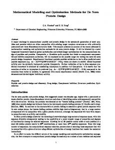
The modeling methods and high-level principles proposed in this paper can aid in the design process of reconfigurable systems. Figure 23 illustrates how they can fit in a general process of designing for reconfigurability. In the first step it is necessary to establish the driving factors for system reconfigurability 共see Fig. 1兲. The identification of the intents allows among other things a value based assessment of the concepts that are generated at a later stage. In the second step, preliminary concepts are generated 共Fig. 4共a兲兲 and are then used as a basis for modeling and evaluating various system states/configurations. The Markov modeling and metacontrol frameworks can be employed toward this end 共Figs. 6 and 16兲. They can also aid in performing trades between few configurations with large reconfiguration bandwidth, 共i.e., the number of elements, n in set A is small and the ␦Ai are large兲 and many configurations with small bandwidths 共n is large while ␦Ai are small兲. The results from the modeling and analysis process, are then used for developing detailed designs of the system. This process can draw from the principles and guidelines that were summarized in the previous section. Once a set of designs is obtained, the evaluation metrics based on the driving requirements 共such as resource efficiency and survivability兲 can then be used for a meaningful comparison 共Figs. 14 and 15兲. This process will be an iterative one in which the designs are refined until the desired goals are satisfied after which the final designs are selected. For large, complex, reconfigurable systems that may exist in several states/configurations, additional research in analytic techniques is required that would be applicable in the detailed design stage of the process. The ultimate objective in the design of any reconfigurable system is driven by the principle of reconfigurability, i.e., the ideal design of a reconfigurable system would be one in which each state/configuration matches closely with an corresponding optimally designed fixed system. Collaborative optimization or Bilevel integrated system synthesis 共BLISS兲关51兴 can potentially be employed toward this end. These methods have been used to optimize various subsystems of a complex system. In their application to reconfigurable system design, instead of subsystems the various states or configurations of the system would be improved. The resulting overall design will thus be one in which each state of the system has been optimized within the given constraints.

Acknowledgment This research was supported by the Richard D. DuPont Fellowship, and the National Aeronautics and Space Administration’s Contract No. NNK05OA50C.

Nomenclature pij P共n兲 Cij Fij Ji ␦Ai ␲i共n兲 ⌽共m , n兲

⫽ ⫽ ⫽ ⫽ ⫽ ⫽ ⫽ ⫽

transition probability from State i to j single-step transition probability matrix cost of reconfiguring from State i to j net benefit in transitioning from State i to j system performance in State i online configuration range of State Ai probability of being in State i at time step n multistep transition probability from m to n

References 关1兴 Compendex, http://www.engineeringvillage2.org. 关2兴 Underwood, K., 2004, “FPGA vs. CPUS: Trends in Peak Floating-Point Performance,” Proceedings of the ACM International Symposium on Field Programmable Gate Arrays, Feb. 24, Monterrey, CA. 关3兴 Keymeulen, D., Zebulum, R., Jin, Y., and Stoica, A., 2000, “Fault-Tolerant Evolvable Hardware Using Field-Programmable Transistor Arrays,” IEEE Trans. Reliab., 49共3兲, pp. 305–316. 关4兴 Mondin, M., Presti, L., and Scova, A., 2002, “A software Radio-Based Reconfigurable Transponder for Space Applications,” Wireless Communications and Mobile Computing, 2, pp. 839–845. 关5兴 Cabo, J., Bravo, R., Lopez, E., and Casas, O., “Galileo TTC Transponder: A Multimode In-Orbit Reconfigurable Transponder.” 关6兴 Mehrabi, M., Ulsoy, A., and Koren, Y., 2000, “Reconfigurable Manufacturing

101102-14 / Vol. 130, OCTOBER 2008

Systems: Key to Future Manufacturing,” J. Intell. Manuf., 11, pp. 403–419. 关7兴 Chen, L., Xi, F., and Macwan, A., 2005, “Optimal Module Selection for Preliminary Design of Reconfigurable Machine Tools,” J. Manuf. Sci. Eng., 127, pp. 104–115. 关8兴 Joshi, S. P., Tidwell, Z., Crossley, W. A., and Ramakrishnan, S., 2004, “Comparison of Morphing Wing Strategies Based Upon Aircraft Performance Impacts,” 45th AIAA/ASME/ASCE/AHS/ASC Structures, Structural Dynamics and Materials Conference, April 2004, Palm Springs, CA, paper No. AIAA-20041722. 关9兴 http://www.nextgenaero.com/success_mfx1.html. 关10兴 Miller, J., Guerrero, J., Goldstein, D., and Robinson, T., 2002, “Spaceframe: Modular Spacecraft Building Blocks for Plug and Play Spacecraft,” 16th Annual/USU Conference on Small Satellites, 2002, Logan, UT. 关11兴 de Weck, O. L., Nadir, W., Wong, J., Bounova, G., and Coffee, T., 2005, “Modular Structures for Manned Space Exploration: The Truncated Octahedron as a Building Block,” First Space Exploration Conference: Continuing the Voyage of Discovery, 30 Jan.–1 Feb. 2005, Orlando, FL, Paper No. AIAA2005-2764. 关12兴 Clark, P., and Rilee, M., 2004, “Bees for Ants: Space Mission Applications for the Autonomous Nano Technology Swarm,” AIAA First Intelligent Systems Technical Conference, Sept. 2004, Chicago, IL, Paper No. AIAA-2004-6303. 关13兴 Olewnik, A., Brauen, T., Ferguson, S., and Kemper, L., 2004, “A Framework for Flexible Systems and Its Implementation in Multiattribute Decision Making,” ASME J. Mech. Des., 126, pp. 412–419. 关14兴 Singh, V., Skiles, S., Krager, J., Wood, K., Jensen, D., and Szmerekovsky, A., 2006, “Innovations in Design Through Transformation: A Fundamental Study of Transformation Principles,” ASME International Design Engineering Technical Conferences and Computers and Information in Engineering Conference, Sept. 10–13, 2006, Philadelphia, PA, Paper No. DETC2006-99575. 关15兴 Khire, R., and Messac, A., 2006, “Selection-Integrated Optimization 共SIO兲 Methodology for Optimal Design of Adaptive Systems,” ASME International Design Engineering Technical Conferences and Computers and Information in Engineering Conference, Sept. 10–13, 2006, Philadelphia, PA, Paper No. DETC2006-99322. 关16兴 Dori, D., 2002, Object-Process Methodology, Springer, New York. 关17兴 http://www.spaceagecontrol.com/s050ai.htm. 关18兴 Howard, R., 1971, Dynamic Probabilistic Systems Vol. 1: Markov Models, Wiley & Sons, New York. 关19兴 Bertsekas, D., and Tsitsiklis, J., 2002, Introduction to Probability, Athena Scientific, Belmont, MA. 关20兴 Feller, W., 1968, An Introduction to Probability Theory and Its Applications, Vol. 1, 3rd ed. Wiley & Sons, New York. 关21兴 Siddiqi, A., Iagnemma, K., and de Weck, O., 2006, “Reconfigurability in Planetary Surface Vehicles: Modeling Approaches and Case Study,” J. Br. Interplanet. Soc., 59. 关22兴 Shinners, S., 1967, Techniques of System Engineering, McGraw-Hill, New York. 关23兴 Ferguson, S., and Lewis, K., 2006, “Effective Development of Reconfigurable Systems Using Linear State Feedback Control,” AIAA J., 44共4兲, pp. 868–878. 关24兴 Asl, F., Ulsoy, A., and Koren, Y., 2000, “Dynamic Modeling and Stability of the Reconfiguration of Manufacturing Systems,” Japan-USA Symposium on Flexible Automation, July 23–26, 2000, Ann Arbor, MI. 关25兴 Siddiqi, A., 2006, “Reconfigurability in Space Systems: Architecting Framework and Case Studies,” Ph.D. thesis, Massachusetts Institute of Technology, Cambridge. 关26兴 2006, www.enidine.com. 关27兴 Codrington, A., 2002, Allmodpro. 关28兴 McGray, D., 2004, “Hot Wheels,” Wired Magazine, October. 关29兴 http://www.ni.com/compactrio/about.htm. 关30兴 Walczyk, D., Lakshmikanthan, J., and Kirk, D., 1998, “Development of a Reconfigurable Tool for Forming Aircraft Body Panels,” J. Manuf. Syst., 17共4兲, pp. 287–296. 关31兴 Yim, M., Roufas, K., Duff, D., Zhang, Y., Eldershaw, C., and Homans, S., 2003, “Modular Reconfigurable Robots in Space Applications,” Auton. Rob., 14, pp. 225–237. 关32兴 Clark, P., and Rilee, M., 2004, “Lara: Near Term Reconfiguration Concepts and Components for Lunar Exploration and Exploitation,” 55th International Astronautical Congress, October 4–8, 2004, Vancouver, Canada, Paper No. IAC-04-IAA.3.8.1.08. 关33兴 Schenker, P., 2000, “Reconfigurable Robots for All Terrain Exploration,” Proc. SPIE, 4196, pp. 454–468. 关34兴 Quinn, J., Repairman in Space. 关35兴 Rodgers, L., 2005, “Concepts and Technology Development for the Autonomous Assembly and Reconfiguration of Modular Space Systems,” M.S. thesis, Massachusetts Institute of Technology, Cambridge. 关36兴 Chau, S., Sengupta, A., Tran, T., and Bakhshi, A., 2002, “Ultra Long-Life Spacecraft for Long Duration Space Exploration Missions,” 53rd International Astronautical Congress, October 10–19, 2002, Houston, TX, Paper No. IAC02-U.2.05. 关37兴 Nishinaga, N., Takeuchi, M., and Suzuki, R., 2004, “Reconfigurable Communication Equipment on SmartSat-I,” IEIC Technical Reoprt, Vol. 104, No. 212, pp. 133–134. 关38兴 Simons, R., Chun, D., and Katehi, L., 2001, “Microelectromechanical Systems 共MEMS兲 Actuators for Antenna Reconfigurability,” National Aeronautics and Space Administration, Glenn Research Center, Tech. Rep. No. NASA/CR2001-210612. 关39兴 2006, “Nextgen to Build Morphing UAV,” Flight International, June 6, 2006,



关40兴关41兴

关42兴关43兴

关44兴关45兴

URL: http://www.flightglobal.com/articles/2006/06/06/207057/nextgen-tobuild-morphing-uav.html http://www.aerospaceweb.org/aircraft/fighter/f14/. Wells, V., Rutherford, J., and Corgiat, A., 1999, “Mission and Concept Evaluation for a Multirole, Mission-Adaptable Air Vehicle,” Aircraft Design, 2, pp. 65–80. http://www.nrao.edu/intro.nm_astro.html. Magee, C., and de Weck, O. L., 2004, “Complex System Classification,” 14th Annual International Symposium of the International Council on Systems Engineering (INCOSE), June 21–24, 2004, Toulouse, France. Hauck, S., 1998, “The Future of Reconfigurable Systems,” 5th Canadian Conference on Field Programmable Devices, June 1998, Montreal, Canada. Fricke, E., and Schulz, A., 2003, “Design for Changeability 共DFC兲: Principles to Enable Changes in Systems Throughout Their Entire Lifecycle,” J. Syst. Eng., 8共4兲, pp. 342–359.


关46兴 Siddiqi, A., and de Weck, O., 2006, “Self-Similar Modular Architectures for Reconfigurable Space Systems,” 57th International Astronautical Congress, October 2–6, 2006, Valencia, Spain, Paper No. IAC-06-D1-1.4.03. 关47兴 Johnson, G. W., ed., 1998, LabVIEW Power Programming, McGraw-Hill, New York. 关48兴 Gu, P., Hashemian, M., and Nee, A., 2004, “Adaptable Design,” CIRP Ann., 53共2兲. 关49兴 Nishinaga, N., Ogawa, Y., Takayama, Y., Takahashi, T., Kubooka, T., and Umehara, H., 2003, “Softsat: Reconfigurable Communication Satellite System,” 21st International Communications Satellite Systems Conference and Exhibit, April 15–19, 2003, Yokohama, Japan, Paper No. AIAA-2003-2420. 关50兴 2006, http://www.fueleconomy.gov/feg.fcv_benefits.shtml. 关51兴 Sobieszczanski-Sobieskr, J., Altus, T., Phillips, M., and Sandusky, R., 2003, “Bilevel Integrated System Synthesis for Concurrent and Distributed Processing,” AIAA J., 41共10兲, pp. 1996–2003.

OCTOBER 2008, Vol. 130 / 101102-15
