Virginia Tech. {filip,fengx,cameron ...... the College of Engineering at Virginia Tech. References. 1. ... In Proc. of Supercomputing'2006, Tampa, FL,. November ...
Modeling Multigrain Parallelism on Heterogeneous Multi-core Processors: A Case Study of the Cell BE Filip Blagojevic, Xizhou Feng, Kirk W. Cameron and Dimitrios S. Nikolopoulos Center for High-End Computing Systems Department of Computer Science Virginia Tech {filip,fengx,cameron,dsn}@cs.vt.edu
Abstract. Heterogeneous multi-core processors invest the most significant portion of their transistor budget in customized “accelerator” cores, while using a small number of conventional low-end cores for supplying computation to accelerators. To maximize performance on heterogeneous multi-core processors, programs need to expose multiple dimensions of parallelism simultaneously. Unfortunately, programming with multiple dimensions of parallelism is to date an ad hoc process, relying heavily on the intuition and skill of programmers. Formal techniques are needed to optimize multi-dimensional parallel program designs. We present a model of multi-dimensional parallel computation for steering the parallelization process on heterogeneous multi-core processors. The model predicts with high accuracy the execution time and scalability of a program using conventional processors and accelerators simultaneously. More specifically, the model reveals optimal degrees of multi-dimensional, task-level and data-level concurrency, to maximize performance across cores. We use the model to derive mappings of two full computational phylogenetics applications on a multi-processor based on the IBM Cell Broadband Engine.
1
Introduction
To overcome the performance and power limitations of conventional generalpurpose microprocessors, many high-performance systems off-load computation to special-purpose hardware. These computational accelerators come in many forms, ranging from SIMD co-processors to FPGA boards to chips with multiple specialized cores. We consider a computational accelerator as any programmable device that is capable of speeding up a computation. Examples of high-end systems utilizing computational accelerators are the Cell Broadband Engine from IBM/Sony/Toshiba [1], Cray’s XD1 [2], the Starbridge Hypercomputer [3], and SGI’s FPGA-based NUMA node [4]. The migration of parallel programming models to accelerator-based architectures raises many challenges. Accelerators require platform-specific programming
II
interfaces and re-formulation of parallel algorithms to fully exploit the additional hardware. Furthermore, scheduling code on accelerators and orchestrating parallel execution and data transfers between host processors and accelerators is a non-trivial exercise [5]. Consider the problem of identifying the most appropriate programming model and accelerator configuration for a given parallel application. The simplest way to identify the best combination is to exhaustively measure the execution time of all of the possible combinations of programming models and mappings of the application to the hardware. Unfortunately, this technique is not scalable to large, complex systems, large applications, or applications with behavior that varies significantly with the input. The execution time of a complex application is the function of many parameters. A given parallel application may consist of N phases where each phase is affected differently by accelerators. Each phase can exploit d dimensions of parallelism or any combination thereof such as ILP, TLP, or both. Each phase or dimension of parallelism can use any of m different programming and execution models such as message passing, shared memory, SIMD, or any combination thereof. Accelerator availability or use may consist of c possible configurations, involving different numbers of accelerators. Exhaustive analysis of the execution time for all combinations requires at least N × d × m × c trials with any given input. Models of parallel computation have been instrumental in the adoption and use of parallel systems. Unfortunately, commonly used models [6, 7] are not directly portable to accelerator-based systems. First, the heterogeneous processing common to these systems is not reflected in most models of parallel computation. Second, current models do not capture the effects of multi-grain parallelism. Third, few models account for the effects of using multiple programming models in the same program. Parallel programming at multiple dimensions and with a synthesis of models consumes both enormous amounts of programming effort and significant amounts of execution time, if not handled with care. To overcome these deficits, we present a model for multi-dimensional parallel computation on heterogeneous multi-core processors. Considering that each dimension of parallelism reflects a different degree of computation granularity, we name the model MMGP, for Model of Multi-Grain Parallelism. MMGP is an analytical model which formalizes the process of programming accelerator-based systems and reduces the need for exhaustive measurements. This paper presents a generalized MMGP model for accelerator-based architectures with one layer of host processor parallelism and one layer of accelerator parallelism, followed by the specialization of this model for the Cell Broadband Engine. The input to MMGP is an explicitly parallel program, with parallelism expressed with machine-independent abstractions, using common programming libraries and constructs. Upon identification of a few key parameters of the application derived from micro-benchmarking and profiling of a sequential run, MMGP predicts with reasonable accuracy the execution time with all feasible mappings of the application to host processors and accelerators. MMGP is fast
III
HPU/LM #1
HPU/LM #NHP
Shared Memory / Message Interface
APU/LM #1
APU/LM #2
APU/LM #NAP
Fig. 1. A hardware abstraction of an accelerator-based architecture with two layers of parallelism. Host processing units (HPUs) supply coarse-grain parallel computation across accelerators. Accelerator processing units (APUs) are the main computation engines and may support internally finer grain parallelism. Both HPUs and APUs have local memories and communicate through shared-memory or message-passing. Additional layers of parallelism can be expressed hierarchically in a similar fashion.
and reasonably accurate, therefore it can be used to quickly identify optimal operating points, in terms of the exposed layers of parallelism and the degree of parallelism in each layer, on accelerator-based systems. Experiments with two complete applications from the field of computational phylogenetics on a sharedmemory multiprocessor with two Cell BEs, show that MMGP models parallel execution time of complex parallel codes with multiple layers of task and data parallelism, with mean error in the range of 1%–5%, across all feasible program configurations on the target system. Due to the narrow margin of error, MMGP predicts accurately the optimal mapping of programs to cores for the cases we have studied so far. In the rest of this paper, we establish preliminary background and terminology for introducing MMGP (Section 2), we develop MMGP (Section 3), and we validate MMGP using two computational phylogenetics applications (Section 4). We discuss related work in Section 5 and conclude the paper in Section 6.
2
Modeling Abstractions
In this section we identify abstractions necessary to allow us to define a simple, accurate model of multi-dimensional parallel computation for heterogeneous multi-core architectures. 2.1
Hardware Abstraction
Figure 1 shows our abstraction of a heterogeneous, accelerator-based parallel architecture. In this abstraction, each node consists of multiple host processing units (HPU) and multiple accelerator processing units (APU). Both the HPUs and APUs have local and shared memory. Multiple HPU-APU nodes form a cluster. We model the communication cost for i and j, where i and j are HPUs,
IV
APUs, and/or HPU-APU pairs, using a variant of LogP [6] of point-to-point communication: Ci,j = Oi + L + Oj , (1) where Ci,j is the communication cost, Oi , Oj is the overhead of send and receive respectively, and L is communication latency. 2.2
Program Abstraction
Figure 2 illustrates the program abstraction used by MMGP. We model programs using a variant of the Hierarchical Task Graph (HTG [8]). An HTG represents multiple layers of concurrency with progressively finer granularity when moving from outermost to innermost layers. We use a phased HTG, in which we partition the application into multiple phases of execution and split each phase into nested sub-phases, each modeled as a single, potentially parallel task. The degree of concurrency may vary between tasks and within tasks. Main Process
Task1
Task2 Subtask3
Subtask2
Subtask1
Subtask3
Subtask2
Subtask1
Task1
Task2
Main Process Time
Fig. 2. Program abstraction for two parallel tasks with nested parallelism.
Mapping a workload with nested parallelism as shown in Figure 2 to an accelerator-based multi-core architecture can be challenging. In the general case, any task of any granularity could be mapped to any type combination of HPUs and APUs. The solution space under these conditions can be unmanageable. We confine the solution space by making some assumptions about the program and the hardware. First, we assume that the application exposes all available layers of inherent parallelism to the runtime environment, without however specifying how to map this parallelism to parallel execution vehicles in hardware. Second, we assume hardware configurations consist of a hierarchy of nested resources, even though the actual resources may not be physically nested in the architecture. For instance, the Cell Broadband Engine can be considered as 2 HPUs and 8 APUs, where the two HPUs correspond to the PowerPC dual-thread SMT core and APUs to the synergistic (SPE) accelerator cores. This assumption is reasonable since it represents faithfully current accelerator architectures, where front-end processors off-load computation and data to accelerators. This assumption simplifies modeling of both communication and computation.
V
3
Model of Multi-grain Parallelism
This section provides theoretical rigor to our approach. We begin by modeling sequential execution on the HPU, with part of the computation off-loaded to a single APU. Next, we incorporate multiple APUs in the model, followed by multiple HPUs. 3.1
Modeling sequential execution
As the starting point, we consider an accelerator-based architecture that consists of one HPU and one APU, and a program with one phase decomposed into three sub-phases, a prologue and epilogue running on the HPU, and a main accelerated phase running on the APU, as illustrated in Figure 3. Off-loading computation
Phase_1 HPU_1 shared Memory APU_1 (a) an architecture with one HPU and one APU
Phase_2
Phase_3 (b) an application with three phases
Fig. 3. The sub-phases of a sequential program are readily mapped to HPUs and APUs. In this example, sub-phases 1 and 3 execute on the HPU and sub-phase 2 executes on the APU. HPUs and APUs communicate via shared memory.
incurs additional communication cost, for loading code and data, in the case of a software-managed APU memory hierarchy, and committing results calculated from the APU. We model each of these communication costs with a latency and an overhead at the end-points, as in Equation 1. We assume that APU’s accesses to data during the execution of a procedure are streamed and overlapped with APU computation. This assumption reflects the capability of current streaming architectures, such as the Cell and Merrimac, to aggressively overlap memory latency with computation, using multiple buffers. Due to overlapped memory latency, communication overhead is assumed to be visible only during loading the code and arguments of a procedure on the APU and during committing the result of an off-loaded procedure to memory, or sending the result of an off-loaded procedure from the APU to the HPU. We note that this assumption does not prevent us from incorporating a more detailed model that accurately estimates the non-overlapped and overlapped communication operations in MMGP. We leave this issue as a subject of future work. Communication overhead for offloading the code and arguments of a procedure and signaling the execution of that procedure on the APU are combined in one term (Os ), while the overhead for returning the result of a procedure from the APU to the HPU and committing intermediate results to memory are combined in another term (Or ).
VI
The execution time for the off-loaded sequential execution for sub-phase 2 in Figure 3, can be modeled as: Tof f load (w2 ) = TAP U (w2 ) + Or + Os
(2)
where TAP U (w2 ) is the time needed to complete sub-phase 2 without additional overhead. We can write the total execution time of all three sub-phases as: T = THP U (w1 ) + TAP U (w2 ) + Or + Os + THP U (w3 )
(3)
To reduce complexity, we replace THP U (w1 )+THP U (w3 ) with THP U , TAP U (w2 ) with TAP U , and Os + Or with Oof f load . We can now rewrite Equation 3 as: T = THP U + TAP U + Oof f load
(4)
The program model in Figure 3 is representative of one of potentially many phases in a program. We further modify Equation 4 for a program with N phases: T =
N X
(THP U,i + TAP U,i + Oof f load )
(5)
i=1
3.2
Modeling parallel execution on APUs
Each off-loaded part of a phase may contain fine-grain parallelism, such as tasklevel parallelism in nested procedures or data-level parallelism in loops. This parallelism can be exploited by using multiple APUs for the offloaded workload. Figure 4 shows the execution time decomposition for execution using one APU and two APUs. We assume that the code off-loaded to an APU during phase i, has a part which can be further parallelized across APUs, and a part executed sequentially on the APU. We denote TAP U,i (1, 1) as the execution time of the further parallelized part of the APU code during the ith phase. The first index 1 refers to the use of one HPU thread in the execution. We denote TAP U,i (1, p) as the execution time of the same part when p APUs are used to execute this part during the ith phase. We denote as CAP U,i the non-parallelized part of APU code in phase i. Therefore, we obtain: TAP U,i (1, p) =
TAP U,i (1, 1) + CAP U,i p
(6)
Given that the HPU off-loads to APUs sequentially, there exists a latency gap between consecutive off-loads on APUs. Similarly, there exists a gap between receiving or committing return values from two consecutive off-loaded procedures on the HPU. We denote with g the larger of the two gaps. On a system with p APUs, parallel APU execution will incur an additional overhead as large as p · g. Thus, we can model the execution time in phase i as: Ti (1, p) = THP U,i +
TAP U,i (1, 1) + CAP U,i + Oof f load + p · g p
(7)
VII Overhead associated with offloading (gap) PPE, SPE Computation
HPU
APU
HPU
APU1 APU2
THPU,i (1,2)
THPU,i (1,1)
Offloading gap
Os
Os TAPU,i (1,2)
Ti (1,1) TAPU,i (1,1)
Ti (1,2)
Or
Or
Receiving gap
Time
Time
(a)
(b)
Fig. 4. Parallel APU execution. The HPU (leftmost bar in parts a and b) offloads computations to one APU (part a) and two APUs (part b). The single point-to-point transfer of part a is modeled as overhead plus computation time on the APU. For multiple transfers, there is additional overhead (g), but also benefits due to parallelization. APU4 APU3
HPU
APU1 APU2
HPU Thread 1 HPU Thread 2
1
THPU,i (2,2) Os
2
THPU,i (2,2)
1
Ti (2,2)
Os
2
Ti (2,2)
1
TAPU,i (2,2)
2 TAPU,i
Or (2,2) Or
Fig. 5. Parallel HPU execution. The HPU (center bar) offloads computations to 4 APUs (2 on the right and 2 on the left).
3.3
Modeling parallel execution on HPUs
Since the compute intensive parts of an application are off-loaded to APUs, HPUs are expected to be idle for extended intervals. Therefore, HPU multithreading can be used to reduce idle time on the HPU and provide more sources of work for APUs. Figure 5 illustrates the execution timeline when two threads share an HPU, and each thread off-loads parallel code on two APUs. We use different shade patterns to represent the workload of different threads. For m concurrent HPU threads, where each thread uses p APUs for distributing a single APU task, the execution time of a single off-loading phase can be represented as: k k Tik (m, p) = THP U,i (m, p) + TAP U,i (m, p) + Oof f load + p · g
(8)
where Tik (m, p) is the completion time of the k th HPU thread during the ith phase. Similarly to Equation 6, we can write the APU time of the k-th thread
VIII
in phase i in Equation 8 as: k TAP U,i (m, p) =
TAP U,i (m, 1) + CAP U,i p
(9)
The execution time of each HPU thread is affected by architecture and software factors. For a multi-threaded HPU where threads share on-chip execution resources, these factors include contention between HPU threads for shared resources, context switch overhead related to resource scheduling, and global synchronization between dependent HPU threads. Considering all three factors, we can model the i-th phase of an HPU thread as: k THP U,i (m, p) = αm · THP U,i (1, p) + TCSW + OCOL
(10)
In this equation, TCSW is context switching time on the HPU and OCOL is the time needed for global synchronization. The parameter αm is introduced to account for contention between threads that share resources on the HPU. On SMT and CMP HPUs, such resources typically include one or more levels of the on-chip cache memory. On SMT HPUs in particular, shared resources include also TLBs, branch predictors and instruction slots in the pipeline. Contention between threads often introduces artificial load imbalance due to occasionally unfair hardware policies of allocating resources between threads. Combining Equations (8)-(10) and summarizing all phases, we can write the execution time for MMGP as: TAP U (1, 1) m·p + N · (OOf f load + TCSW + OCOL + p · g)
T (m, p) = αm · THP U (1, 1) + + CAP U
(11)
Due to limited hardware resources (i.e. number of HPUs and APUs), we further constrain this equation to m × p ≤ NAP U , where NAP U is the number of available APUs. As described later in this paper, we can either measure directly or estimate all parameters in Equation 11 from micro-benchmarks and a profile of a sequential run of the program. Given a parallel program, MMGP can be applied using the following process: 1. Estimate OOf f load , αm , TCSW and OCOL using micro-benchmarks. 2. Profile a run of the sequential program, with annotations of parallelism included, to estimate THP U (1), TAP U (1, 1) and CAP U . 3. Solve a special case of Equation 11 (e.g. 7) to find the optimal mapping between application concurrency and available HPUs and APUs.
4
Experimental Validation and Results
We use MMGP to derive multi-dimensional parallelization schemes for two bioinformatics applications, RAxML and PBPI, on an IBM QS20 BladeCenter with two Cell BEs. RAxML and PBPI construct evolutionary trees from DNA or AA sequences, using different optimality criteria for approximating the best trees.
IX
4.1
Parameter Approximation
MMGP has six free parameters, CAP U , Oof f load , g, TCSW , OCOL and αm . We estimate four of the parameters using micro-benchmarks. αm captures contention between processes or threads running on the PPE. This contention depends on the scheduling algorithm on the PPE. We estimate αm under an event-driven scheduling model which oversubscribes the PPE with more processes than the number of hardware threads supported for simultaneous execution on the PPE, and switches between processes upon each off-loading event on the PPE [5]. The reason for using oversubscribing is the potential imbalance between supply and demand of computation between the PPE and SPEs. To estimate αm , we use a parallel micro-benchmark that computes the product of two M × M arrays of double-precision floating point elements. Matrixmatrix multiplication involves O(n3 ) computation and O(n2 ) data transfers, thus stressing the impact of sharing execution resources and the L1 and L2 caches between processes on the PPE. We used several different matrix sizes, ranging from 100×100 to 500×500, to exercise different levels of pressure on the thread-shared caches of the PPE. In the MMGP model, we use αm =1.28, computed from these experiments. We should point out that αm is not a constant in the general case. However, αm affects only a small portion of the code (executed on the HPU). Therefore, approximating αm with a constant is a reasonable choice which results in fairly accurate MMGP predictions, as shown later in this section. PPE-SPE communication is optimally implemented through DMAs on Cell. In PBPI and RAxML, the off-loaded code remains in the local storage during the entire execution of the application. Also, the arguments for the off-loaded functions are fetched directly from the main memory by the SPE thread. Therefore, the only PPE-SPE communication (Oof f load ) is PPE → SPE trigger signal, and the signal sent back by each SPE after finishing the off-loaded work. We devised a ping-pong micro-benchmark using DMAs to send a single integer from the PPE to one SPE and backwards. We measured PPE→SPE→PPE round-trip communication overhead for a single 4-byte packet to 70 ns. To measure the overhead caused by various collective communications we used mpptest [9] on the PPE. Using a micro-benchmark that repeatedly executes the sched yield() system call, we estimate the overhead caused by the context switching (TCSW ) on the PPE to 2 µs. CAP U and the gap g between consecutive DMAs on the PPE are applicationdependent and can not be approximated easily with a micro-benchmark. To estimate these parameters, we use a profile of a sequential run of the code, with tasks off-loaded on one SPE. 4.2
PBPI Outline
PBPI [10, 11] is a parallel Bayesian phylogenetic inference implementation, which constructs phylogenetic trees from DNA or AA sequences using a Markov chain Monte Carlo sampling method. The method exploits the multi-dimensional data parallelism available in Bayesian phylogenetic inference (across the sequence
X
and within the likelihood computations), to achieve scalability on large-scale distributed memory systems, such as the IBM BlueGene/L [12]. The algorithm used in PBPI can be summarized as follows: 1. Markov chains are partitioned into chain groups and the data set is split into segments along the sequences. 2. Virtual processors are organized in a two-dimensional grid; each chain group is mapped to one row on the grid, and each segment is mapped to one column on the grid. 3. During each generation, the partial likelihood across all columns is computed using all-to-all communication to collect the complete likelihood values from all virtual processors on the same row. 4. When there are multiple chains, two chains are randomly chosen for swapping using point-to-point communication. PBPI is implemented in MPI. We ported PBPI to Cell by off-loading the computationally expensive functions that perform the likelihood calculation on SPEs and applied a sequence of Cell-specific optimizations on the off-loaded code. 4.3
PBPI with One Dimension of Parallelism
We compare the PBPI execution times modeled by MMGP to the actual execution times obtained on real hardware, using various degrees of PPE and SPE parallelism, the equivalents of HPU and APU parallelism on Cell. For these experiments, we used the arch107 L10000 input data set. This data set consists of 107 sequences, each with 10000 characters. We run PBPI with one Markov chain for 20000 generations. Using the time base register on the PPE and the decrementer register on one SPE, we were able to profile the sequential execution of the program. We obtained the following model parameters for PBPI: THP U = 1.3s, TAP U = 370s, g = 0.8s and CAP U = 1.72s. Figure 6 (a),(b), compares modeled and actual execution times for PBPI, when PBPI only exploits one-dimensional PPE (HPU) parallelism in which each PPE thread uses one SPE for off-loading. We execute the code with up to 16 MPI processes, which off-load code to up to 16 SPEs on two Cell BEs. Referring to Equation 11, we set p = 1 and vary the value of m from 1 to 16. The X-axis shows the number of processes running on the PPE (i.e. HPU parallelism), and the Y-axis shows the modeled and measured execution times. The maximum prediction error of MMGP is 5%. The arithmetic mean of the error is 2.3% and the standard deviation is 1.4. The largest gap between MMGP prediction and the real execution time occurs when the number of processes is larger than 10, (Figure 6 (b)). The reason is contention caused by context switching and MPI communication, when a large number of processes is multiplexed on 2 PPEs. Nevertheless, the maximum prediction error even in this case is close to 5%. Figure 6 (c),(d), illustrates modeled and actual execution times when PBPI uses one dimension of SPE (APU) parallelism. Referring to Equation 11, we set m = 1 and vary p from 1 to 16. MMGP remains accurate, the mean prediction
XI
(a)
(b)
(c)
(d)
Fig. 6. MMGP predictions and actual execution times of PBPI, when the code uses one dimension of PPE-HPU, ((a), (b)), and SPE-APU ((c), (d)) parallelism.
error is 4.1% and the standard deviation is 3.2. The maximum prediction error in this case is 10%. We measured the execution time necessary for solving Equation 11 for T (m, p) to be 0.4µs. The overhead of the model is therefore negligible. 4.4
PBPI with Two Dimensions of Parallelism
Figure 7 shows the modeled and actual execution times of PBPI for all feasible combinations of two-dimensional parallelism under the constraint that the code does not use more than 16 SPEs, i.e. the maximum number of SPEs on the experimental platform. MMGP’s mean prediction error is 3.2%, the standard deviation of the error is 2.6 and the maximum prediction error is 10%. The important observation in these results is that MMGP matches the experimental outcome in terms of the degrees of PPE and SPE parallelism to use in PBPI for maximizing performance. In a real program development scenario, MMGP would point the programmer in the direction of using two layers of parallelism with a balanced allocation of PPE contexts and SPEs between the two layers. In principle, if the difference between the optimal and nearly optimal configurations of parallelism are within the margin of error of MMGP, MMGP may not predict the optimal configuration accurately. In the applications we tested, MMGP never mispredicts the optimal configuration. We also anticipate that due to high accuracy, potential MMGP mispredictions should generally lead to configurations that perform marginally lower than the actual optimal configuration. 4.5
RAxML Outline
RAxML uses an embarrassingly parallel master-worker algorithm, implemented with MPI. In RAxML, workers perform two tasks: (i) calculation of multiple inferences on the initial alignment in order to determine the best known Maximum Likelihood tree, and (ii) bootstrap analyses to determine how well supported are some parts of the Maximum Likelihood tree. From a computational point of view, inferences and bootstraps are identical. We use an optimized port of RAxML on Cell, described in further detail in [5].
XII
400
Execution time in seonds
350 MMGP model Measured time
300 250 200 150 100 50
(1,1) (1,2) (2,1) (1,3) (3,1) (1,4) (2,2) (4,1) (1,5) (5,1) (1,6) (2,3) (3,2) (6,1) (1,7) (7,1) (1,8) (2,4) (4,2) (8,1) (1,9) (3,3) (9,1) (1,10) (2,5) (5,2) (10,1) (1,11) (11,1) (1,12) (2,6) (3,4) (4,3) (6,2) (12,1) (1,13) (13,1) (1,14) (2,7) (7,2) (14,1) (1,15) (3,5) (5,3) (15,1) (1,16) (2,8) (4,4) (8,2) (16,1)
0
Executed Configuration (#PPE,#SPE)
Fig. 7. MMGP predictions and actual execution times of PBPI, when the code uses two dimensions of SPE (APU) and PPE (HPU) parallelism. Performance is optimized with a layer of 4-way PPE parallelism and a nested layer of 4-way SPE parallelism.
4.6
RAxML with Two Dimensions of Parallelism
We compare the execution time of RAxML to the time modeled by MMGP, using a data set that contains 10 organisms, each represented by a DNA sequence of 50,000 nucleotides. We set RAxML to perform a total of 16 bootstraps using different parallel configurations. The MMGP parameters for RAxML, obtained from profiling a sequential run of the code are THP U = 8.8s, TAP U = 118s, CAP U = 157s. The values of other MMGP parameters are negligible compared to TAP U , THP U , and CAP U , therefore we disregard them for RAxML. We observe that a large portion of the off-loaded RAxML code cannot be parallelized across SPEs (CAP U - 57% of the total SPE time). Due to this limitation, RAxML does not scale with one-dimensional parallel configurations that use more than 8 SPEs. We omit the results comparing MMGP and measured time in RAxML with one dimension of parallelism due to space limitations. MMGP remains highly accurate when one dimension of parallelism is exploited in RAxML, with mean error rates of 3.4% for configurations with only PPE parallelism and 2% for configurations with only SPE parallelism. Figure 8 shows the actual and modeled execution times in RAxML, when the code exposes two dimensions of parallelism to the system. Regardless of execution time prediction accuracy, MMGP is able to pin-point the optimal parallelization model thanks to the low prediction error. Performance is optimized in the case of RAxML with task-level parallelization and no further data-parallel decomposition of tasks between SPEs. There is very little opportunity for scalable data-level parallelization in RAxML. MMGP remains very accurate, with mean execution time prediction error of 2.8%, standard deviation of 1.9, and maximum prediction error of 7%.
XIII
Execution time in seconds
350
MMGP model Measured time
300 250 200 150 100 50
(2,8)
(16,1)
(8,2)
(2,7)
(4,3)
(2,6)
(2,5)
(8,1)
(4,2)
(2,4)
(1,8)
(1,7)
(2,3)
(1,6)
(1,5)
(4,1)
(2,2)
(1,4)
(1,3)
(2,1)
(1,2)
(1,1)
0
Executed configuration (#PPE/#SPE)
Fig. 8. MMGP predictions and actual execution times of RAxML, when the code uses two dimensions of SPE (APU) and PPE (HPU) parallelism. Performance is optimized by oversubscribing the PPE and maximizing task-level parallelism.
Although the two codes tested are similar in their computational objective, their optimal parallelization model is at the opposite ends of the design spectrum. MMGP accurately reflects this disparity, using a small number of parameters and rapid prediction of execution times across a large number of feasible program configurations.
5
Related Work
Traditional parallel programming models, such as BSP [13], LogP [6], and derived models [14, 15] developed to respond to changes in the relative impact of architectural components on the performance of parallel systems, are based on a minimal set of parameters, to capture the impact of communication overhead on computation running across a homogeneous collection of interconnected processors. MMGP borrows elements from LogP and its derivatives, to estimate performance of parallel computations on heterogeneous parallel systems with multiple dimensions of parallelism implemented in hardware. A variation of LogP, HLogP [7], considers heterogeneous clusters with variability in the computational power and interconnection network latencies and bandwidths between the nodes. Although HLogP is applicable to heterogeneous multi-core architectures, it does not consider nested parallelism. It should be noted that although MMGP has been evaluated on architectures with heterogeneous processors, it can also support architectures with heterogeneity in their communication substrates. Several parallel programming models have been developed to support nested parallelism, including extensions of common parallel programming libraries such as MPI and OpenMP to support nested parallel constructs [16, 17]. Prior work on languages and libraries for nested parallelism based on MPI and OpenMP is largely based on empirical observations on the relative speed of data communication via cache-coherent shared memory, versus communication with message
XIV
passing through switching networks. Our work attempts to formalize these observations into a model which seeks optimal work allocation between layers of parallelism in the application and optimal mapping of these layers to heterogeneous parallel execution hardware. Sharapov et. al [18] use a combination of queuing theory and cycle-accurate simulation of processors and interconnection networks, to predict the performance of hybrid parallel codes written in MPI/OpenMP on ccNUMA architectures. MMGP uses a simpler model, designed to estimate scalability along more than one dimensions of parallelism on heterogeneous parallel architectures.
6
Conclusions
The introduction of accelerator-based parallel architectures complicates the problem of mapping algorithms to systems, since parallelism can no longer be considered as a one-dimensional abstraction of processors and memory. We presented a new model of multi-dimensional parallel computation, MMGP, which we introduced to relieve users from the arduous task of mapping parallelism to accelerator-based architectures. We have demonstrated that the model is fairly accurate, albeit simple, and that it is extensible and easy to specialize for a given architecture. We envision three uses of MMGP: i) As a rapid prototyping tool for porting algorithms to accelerator-based architectures. ii) As a compiler tool for assisting compilers in deriving efficient mappings of programs to acceleratorbased architectures automatically. iii) As a runtime tool for dynamic control of parallelism in applications. Extensions of MMGP which we will explore in future research include accurate modeling of non-overlapped communication and memory accesses, accurate modeling of SIMD and instruction-level parallelism within accelerators, integration of the model with runtime performance prediction and optimization techniques, and application of the model to emerging acceleratorbased parallel systems.
Acknowledgments This research is supported by the National Science Foundation (Grant CCF0346867, CCF-0715051), the U.S. Department of Energy (Grants DE-FG0205ER25689, DE-FG02-06ER25751), the Barcelona Supercomputing Center, and the College of Engineering at Virginia Tech.
References 1. IBM Corporation. Cell Broadband Engine Architecture, Version 1.01. Technical report, October 2006. 2. M. Fahey, S. Alam, T. Dunigan, J. Vetter, and P. Worley. Early Evaluation of the Cray XD1. In Proc. of the 2005 Cray Users Group Meeting, 2005. 3. Starbridge Systems. A Reconfigurable Computing Model for Biological Research: Application of Smith-Waterman Analysis to Bacterial Genomes. Technical report, 2005.
XV 4. R. Chamberlain, S. Miller, J. White, and D. Gall. Highly-Scalable Recondigurable Computing. In Proc. of the 2005 MAPLD International Conference, Washington, DC, September 2005. 5. F. Blagojevic, D. Nikolopoulos, A. Stamatakis, and C. Antonopoulos. Dynamic Multigrain Parallelization on the Cell Broadband Engine. In Proc. of the 2007 ACM SIGPLAN Symposium on Principles and Practice of Parallel Programming, pages 90–100, San Jose, CA, March 2007. 6. D. Culler, R. Karp, D. Patterson, A. Sahay, K. Scauser, E. Santos, R. Subramonian, and T. Von Eicken. LogP: Towards a Realistic Model of Parallel Computation. In Proc. of the 4th ACM SIGPLAN Symposium on Principles and Practice of Parallel Programming (PPoPP’93), May 1993. 7. J. Bosque and L. Pastor. A Parallel Computational Model for Heterogeneous Clusters. IEEE Transactions on Parallel and Distributed Systems, 17(12):1390– 1400, December 2006. 8. M. Girkar and C. Polychronopoulos. The Hierarchical Task Graph as a Universal Intermediate Representation. International Journal of Parallel Programming, 22(5):519–551, October 1994. 9. W. Gropp and E. Lusk. Reproducible Measurements of MPI Performance Characteristics. In Proc. of the 6th European PVM/MPI User’s Group Meeting, pages 11–18, Barcelona, Spain, September 1999. 10. X. Feng, K. Cameron, and D. Buell. PBPI: a high performance Implementation of Bayesian Phylogenetic Inference. In Proc. of Supercomputing’2006, Tampa, FL, November 2006. 11. X. Feng, D. Buell, J. Rose, and P. Waddell. Parallel algorithms for bayesian phylogenetic inference. Journal of Parallel Distributed Computing, 63(7-8):707–718, 2003. 12. X. Feng, K. Cameron, B. Smith, and C. Sosa. Building the Tree of Life on Terascale Systems. In Proc. of the 21st International Parallel and Distributed Processing Symposium, Long Beach, CA, March 2007. 13. L. Valiant. A bridging model for parallel computation. Communications of the ACM, 22(8):103–111, August 1990. 14. K. Cameron and X. Sun. Quantifying Locality Effect in Data Access Delay: Memory LogP. In Proc. of the 17th International Parallel and Distributed Processing Symposium, Nice, France, April 2003. 15. A. Alexandrov, M. Ionescu, C. Schauser, and C. Scheiman. LogGP: Incorporating Long Messages into the LogP Model: One Step Closer towards a Realistic Model for Parallel Computation. In Proc. of the 7th Annual ACM Symposium on Parallel Algorithms and Architectures, pages 95–105, Santa Barbara, CA, June 1995. 16. F. Cappello and D. Etiemble. MPI vs. MPI+OpenMP on the IBM SP for the NAS Benchmarks. In Proc. of the IEEE/ACM Supercomputing’2000: High Performance Networking and Computing Conference (SC’2000), Dallas, Texas, November 2000. 17. G. Krawezik. Performance Comparison of MPI and three OpenMP Programming Styles on Shared Memory Multiprocessors. In Proc. of the 15th Annual ACM Symposium on Parallel Algorithms and Architectures, June 2003. 18. I. Sharapov, R. Kroeger, G. Delamater, R. Cheveresan, and M. Ramsay. A Case Study in Top-Down Performance Estimation for a Large-Scale Parallel Application. In Proc. of the 11th ACM SIGPLAN Symposium on Pronciples and Practice of Parallel Programming, pages 81–89, New York, NY, March 2006.